KPLS

KPLS is a kriging model that uses the partial least squares (PLS) method. KPLS is faster than kriging because of the low number of hyperparameters to be estimated while maintaining a good accuracy. This model is suitable for high-dimensional problems due to the kernel constructed through the PLS method. The PLS method [1] is a well known tool for high-dimensional problems that searches the direction that maximizes the variance between the input and output variables. This is done by a projection in a smaller space spanned by the so-called principal components. The PLS information are integrated into the kriging correlation matrix to scale the number of inputs by reducing the number of hyperparameters. The number of principal components \(h\) , which corresponds to the number of hyperparameters for KPLS and much lower than \(nx\) (number of dimension of the problem), usually does not exceed 4 components:

\[\begin{split}\prod\limits_{l=1}^{nx}\exp\left(-\theta_l\left(x_l^{(i)}-x_l^{(j)}\right)^2\right),\qquad \qquad \qquad \prod\limits_{k=1}^h \prod\limits_{l=1}^{nx} \exp\left(-\theta_k\left(w_{*l}^{(k)}x_l^{(i)}-w_{*l}^{(k)}x_l^{(j)}\right)^{2}\right) \quad \forall\ \theta_l,\theta_k\in\mathbb{R}^+\\ \text{Standard Gaussian correlation function} \quad \qquad\text{PLS-Gaussian correlation function}\qquad \qquad\qquad\quad\end{split}\]

Both absolute exponential and squared exponential kernels are available for KPLS model. More details about the KPLS approach could be found in these sources [2].

For an automatic selection of the number of components \(h\), the adjusted Wold’s R criterion is implemented as detailed in [3].

[1]

Wold, H., Soft modeling by latent variables: the nonlinear iterative partial least squares approach, Perspectives in probability and statistics, papers in honour of MS Bartlett, 1975, pp. 520–540.

[2]

Bouhlel, M. A. and Bartoli, N. and Otsmane, A. and Morlier, J., Improving kriging surrogates of high-dimensional design models by Partial Least Squares dimension reduction, Structural and Multidisciplinary Optimization, Vol. 53, No. 5, 2016, pp. 935–952.

[3]

Saves, P. and Bartoli, N. and Diouane, Y. and Lefebvre, T. and Morlier, J. and David, C. and Nguyen Van, E. and Defoort, S., Bayesian optimization for mixed variables using an adaptive dimension reduction process: applications to aircraft design, AIAA SCITECH 2022 Forum, pp. 0082.

Usage

import matplotlib.pyplot as plt
import numpy as np

from smt.surrogate_models import KPLS

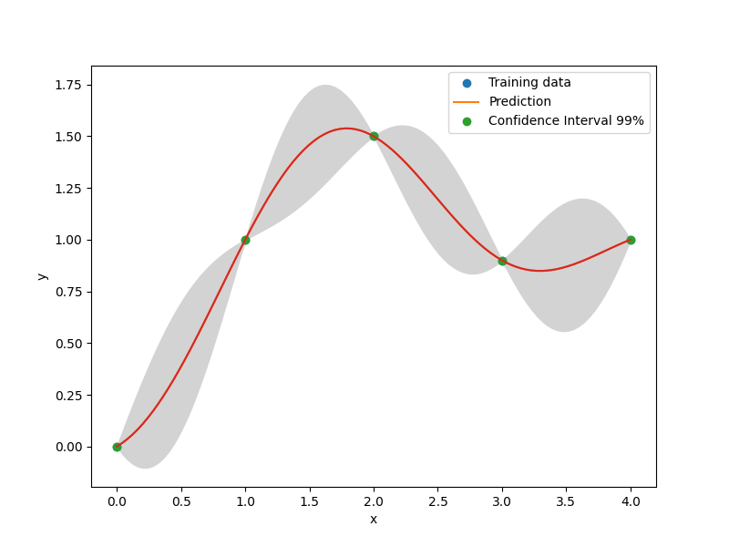
xt = np.array([0.0, 1.0, 2.0, 3.0, 4.0])
yt = np.array([0.0, 1.0, 1.5, 0.9, 1.0])

sm = KPLS(theta0=[1e-2])
sm.set_training_values(xt, yt)
sm.train()

num = 100
x = np.linspace(0.0, 4.0, num)
y = sm.predict_values(x)
# estimated variance
# add a plot with variance
s2 = sm.predict_variances(x)
# to compute the derivative according to the first variable
_dydx = sm.predict_derivatives(xt, 0)

plt.plot(xt, yt, "o")
plt.plot(x, y)
plt.xlabel("x")
plt.ylabel("y")
plt.legend(["Training data", "Prediction"])
plt.show()

plt.plot(xt, yt, "o")
plt.plot(x, y)
plt.fill_between(
    np.ravel(x),
    np.ravel(y - 3 * np.sqrt(s2)),
    np.ravel(y + 3 * np.sqrt(s2)),
    color="lightgrey",
)
plt.xlabel("x")
plt.ylabel("y")
plt.legend(["Training data", "Prediction", "Confidence Interval 99%"])
plt.show()

___________________________________________________________________________

                                   KPLS
___________________________________________________________________________

 Problem size

      # training points.        : 5

___________________________________________________________________________

 Training

   Training ...
   Training - done. Time (sec):  0.0968523
___________________________________________________________________________

 Evaluation

      # eval points. : 100

   Predicting ...
   Predicting - done. Time (sec):  0.0002611

   Prediction time/pt. (sec) :  0.0000026

___________________________________________________________________________

 Evaluation

      # eval points. : 5

   Predicting ...
   Predicting - done. Time (sec):  0.0003815

   Prediction time/pt. (sec) :  0.0000763

Usage with an automatic number of components

import numpy as np

from smt.problems import TensorProduct
from smt.sampling_methods import LHS
from smt.surrogate_models import KPLS

# The problem is the exponential problem with dimension 10
ndim = 10
prob = TensorProduct(ndim=ndim, func="exp")

sm = KPLS(
    eval_n_comp=True,
    eval_n_comp_strategy="wold",
)
samp = LHS(xlimits=prob.xlimits, seed=42)
xt = samp(50)
yt = prob(xt)
sm.set_training_values(xt, yt)
sm.train()

## The model automatically choose a dimension of 5
ncomp = sm.options["n_comp"]
print("\n The model automatically choose " + str(ncomp) + " components.")

## You can predict a 10-dimension point from the 3-dimensional model
print(
    sm.predict_values(
        np.array([[-0.9, -0.7, -0.5, -0.3, -0.1, 0.1, 0.3, 0.5, 0.7, 0.9]])
    )
)
print(
    sm.predict_variances(
        np.array([[-0.9, -0.7, -0.5, -0.3, -0.1, 0.1, 0.3, 0.5, 0.7, 0.9]])
    )
)

___________________________________________________________________________

                                   KPLS
___________________________________________________________________________

 Problem size

      # training points.        : 50

___________________________________________________________________________

 Training

   Training ...
   Training - done. Time (sec): 87.2217591

 The model automatically choose 5 components.
___________________________________________________________________________

 Evaluation

      # eval points. : 1

   Predicting ...
   Predicting - done. Time (sec):  0.0002754

   Prediction time/pt. (sec) :  0.0002754

[[2.73415724]]
[[40.38142747]]

Usage with a range of number of components

import numpy as np

from smt.problems import TensorProduct
from smt.sampling_methods import LHS
from smt.surrogate_models import KPLS

# The problem is the exponential problem with dimension 10
ndim = 10
prob = TensorProduct(ndim=ndim, func="exp")

n_comp_range = [2, 6]  # We explore the range [1, 5] n_dim and we chose the best

sm = KPLS(
    eval_n_comp=True,
    eval_n_comp_strategy="exhaustive",
    range_n_comp_exhaustive=n_comp_range,
)
samp = LHS(xlimits=prob.xlimits, seed=42)
xt = samp(50)
yt = prob(xt)
sm.set_training_values(xt, yt)
sm.train()

## The model automatically choose a dimension of 5
ncomp = sm.options["n_comp"]
print("\n The model automatically choose " + str(ncomp) + " components.")

## You can predict a 10-dimension point from the 3-dimensional model
print(
    sm.predict_values(
        np.array([[-0.9, -0.7, -0.5, -0.3, -0.1, 0.1, 0.3, 0.5, 0.7, 0.9]])
    )
)
print(
    sm.predict_variances(
        np.array([[-0.9, -0.7, -0.5, -0.3, -0.1, 0.1, 0.3, 0.5, 0.7, 0.9]])
    )
)

___________________________________________________________________________

                                   KPLS
___________________________________________________________________________

 Problem size

      # training points.        : 50

___________________________________________________________________________

 Training

   Training ...
   Training - done. Time (sec): 59.3835318

 The model automatically choose 5 components.
___________________________________________________________________________

 Evaluation

      # eval points. : 1

   Predicting ...
   Predicting - done. Time (sec):  0.0003910

   Prediction time/pt. (sec) :  0.0003910

[[2.73416137]]
[[40.38140393]]

Options

List of options

Option	Default	Acceptable values	Acceptable types	Description
print_global	True	None	[‘bool’]	Global print toggle. If False, all printing is suppressed
print_training	True	None	[‘bool’]	Whether to print training information
print_prediction	True	None	[‘bool’]	Whether to print prediction information
print_problem	True	None	[‘bool’]	Whether to print problem information
print_solver	True	None	[‘bool’]	Whether to print solver information
poly	constant	[‘constant’, ‘linear’, ‘quadratic’]	[‘str’]	Regression function type
corr	squar_exp	[‘abs_exp’, ‘squar_exp’, ‘pow_exp’]	[‘str’]	Correlation function type
pow_exp_power	1.9	None	[‘float’]	Power for the pow_exp kernel function (valid values in (0.0, 2.0]). This option is set automatically when corr option is squar, abs, or matern.
categorical_kernel	MixIntKernelType.CONT_RELAX	[<MixIntKernelType.CONT_RELAX: ‘CONT_RELAX’>, <MixIntKernelType.GOWER: ‘GOWER’>, <MixIntKernelType.EXP_HOMO_HSPHERE: ‘EXP_HOMO_HSPHERE’>, <MixIntKernelType.HOMO_HSPHERE: ‘HOMO_HSPHERE’>, <MixIntKernelType.COMPOUND_SYMMETRY: ‘COMPOUND_SYMMETRY’>, <MixIntKernelType.DIST_ENCODING: ‘DIST_ENCODING’>]	None	The kernel to use for categorical inputs. Only for non continuous Kriging
categorical_kernel_beta	1.0	None	[‘float’, ‘int’]	Power for the distributional encoding kernel (valid values in (0.0, 2.0]).
hierarchical_kernel	MixHrcKernelType.ALG_KERNEL	[<MixHrcKernelType.ALG_KERNEL: ‘ALG_KERNEL’>, <MixHrcKernelType.ARC_KERNEL: ‘ARC_KERNEL’>]	None	The kernel to use for mixed hierarchical inputs. Only for non continuous Kriging
nugget	2.220446049250313e-14	None	[‘float’]	a jitter for numerical stability
theta0	[0.01]	None	[‘list’, ‘ndarray’]	Initial hyperparameters
theta_bounds	[1e-06, 20.0]	None	[‘list’, ‘ndarray’]	bounds for hyperparameters
hyper_opt	TNC	[‘Cobyla’, ‘TNC’, ‘NoOp’]	None	Optimiser for hyperparameters optimisation
eval_noise	False	[True, False]	[‘bool’]	noise evaluation flag
noise0	[0.0]	None	[‘list’, ‘ndarray’]	Initial noise hyperparameters
noise_bounds	[np.float64(2.220446049250313e-14), 10000000000.0]	None	[‘list’, ‘ndarray’]	bounds for noise hyperparameters
use_het_noise	False	[True, False]	[‘bool’]	heteroscedastic noise evaluation flag
n_start	10	None	[‘int’]	number of optimizer runs (multistart method)
xlimits	None	None	[‘list’, ‘ndarray’]	definition of a design space of float (continuous) variables: array-like of size nx x 2 (lower, upper bounds)
design_space	None	None	[‘BaseDesignSpace’, ‘list’, ‘ndarray’]	definition of the (hierarchical) design space: use smt.design_space.DesignSpace as the main API. Also accepts list of float variable bounds
is_ri	False	None	[‘bool’]	activate reinterpolation for noisy cases
seed	41	None	[‘NoneType’, ‘int’, ‘Generator’]	Numpy Generator object or seed number which controls random draws for internal optim (set by default to get reproductibility)
n_comp	1	None	[‘int’]	Number of principal components. Only used when eval_n_comp=False. Ignored when eval_n_comp=True (the optimal value is estimated instead).
eval_n_comp	False	[True, False]	[‘bool’]	If True, the optimal number of components is estimated automatically using the strategy defined by eval_n_comp_strategy. If False, the value of n_comp is used directly.
eval_comp_treshold	1.0	None	[‘float’]	Threshold for Wold’s R criterion (used when eval_n_comp_strategy=’wold’).
eval_n_comp_strategy	wold	[‘wold’, ‘exhaustive’]	[‘str’]	Strategy used to estimate the optimal number of components when eval_n_comp=True. ‘wold’: increments n_comp until the cross-validation error stops decreasing (early stopping via Wold’s R criterion). ‘exhaustive’: evaluates all values in range_n_comp_exhaustive and picks the global minimum.
range_n_comp_exhaustive	None	None	[‘list’, ‘tuple’, ‘ndarray’, ‘NoneType’]	Search range [n_min, n_max] (inclusive) for the exhaustive strategy. Only used when eval_n_comp=True and eval_n_comp_strategy=’exhaustive’. If None, defaults to [1, max(1, n_features // 10)].
cat_kernel_comps	None	None	[‘list’]	Number of components for PLS categorical kernel