Multi-Fidelity Kriging (MFK)

MFK is a multi-fidelity modeling method which uses an autoregressive model of order 1 (AR1).

\[y_\text{high}({\bf x})=\rho(x) \cdot y_\text{low}({\bf x}) + \delta({\bf x})\]

where \(\rho(x)\) is a scaling/correlation factor (constant, linear or quadratic) and \(\delta(\cdot)\) is a discrepancy function.

The additive AR1 formulation was first introduced by Kennedy and O’Hagan [1]. The implementation here follows the one proposed by Le Gratiet [2]. It offers the advantage of being recursive, easily extended to \(n\) levels of fidelity and offers better scaling for high numbers of samples. This method only uses nested sampling training points as described by Le Gratiet [2].

References

[1]

Kennedy, M.C. and O’Hagan, A., Bayesian calibration of computer models. Journal of the Royal Statistical Society. 2001

[2] (1,2)

Le Gratiet, L., Multi-fidelity Gaussian process regression for computer experiments. PhD Thesis. 2013

Usage

import numpy as np
import matplotlib.pyplot as plt
from smt.applications.mfk import MFK, NestedLHS

# low fidelity model
def lf_function(x):
    import numpy as np

    return (
        0.5 * ((x * 6 - 2) ** 2) * np.sin((x * 6 - 2) * 2)
        + (x - 0.5) * 10.0
        - 5
    )

# high fidelity model
def hf_function(x):
    import numpy as np

    return ((x * 6 - 2) ** 2) * np.sin((x * 6 - 2) * 2)

# Problem set up
xlimits = np.array([[0.0, 1.0]])
xdoes = NestedLHS(nlevel=2, xlimits=xlimits, random_state=0)
xt_c, xt_e = xdoes(7)

# Evaluate the HF and LF functions
yt_e = hf_function(xt_e)
yt_c = lf_function(xt_c)

sm = MFK(theta0=xt_e.shape[1] * [1.0])

# low-fidelity dataset names being integers from 0 to level-1
sm.set_training_values(xt_c, yt_c, name=0)
# high-fidelity dataset without name
sm.set_training_values(xt_e, yt_e)

# train the model
sm.train()

x = np.linspace(0, 1, 101, endpoint=True).reshape(-1, 1)

# query the outputs
y = sm.predict_values(x)
_mse = sm.predict_variances(x)
_derivs = sm.predict_derivatives(x, kx=0)

plt.figure()

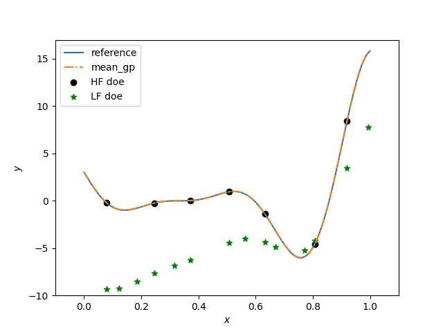
plt.plot(x, hf_function(x), label="reference")
plt.plot(x, y, linestyle="-.", label="mean_gp")
plt.scatter(xt_e, yt_e, marker="o", color="k", label="HF doe")
plt.scatter(xt_c, yt_c, marker="*", color="g", label="LF doe")

plt.legend(loc=0)
plt.ylim(-10, 17)
plt.xlim(-0.1, 1.1)
plt.xlabel(r"$x$")
plt.ylabel(r"$y$")

plt.show()

___________________________________________________________________________

                                    MFK
___________________________________________________________________________

 Problem size

      # training points.        : 7

___________________________________________________________________________

 Training

   Training ...
   Training - done. Time (sec):  0.4344051
___________________________________________________________________________

 Evaluation

      # eval points. : 101

   Predicting ...
   Predicting - done. Time (sec):  0.0002229

   Prediction time/pt. (sec) :  0.0000022

___________________________________________________________________________

 Evaluation

      # eval points. : 101

   Predicting ...
   Predicting - done. Time (sec):  0.0001872

   Prediction time/pt. (sec) :  0.0000019

Options

List of options

Option	Default	Acceptable values	Acceptable types	Description
print_global	True	None	[‘bool’]	Global print toggle. If False, all printing is suppressed
print_training	True	None	[‘bool’]	Whether to print training information
print_prediction	True	None	[‘bool’]	Whether to print prediction information
print_problem	True	None	[‘bool’]	Whether to print problem information
print_solver	True	None	[‘bool’]	Whether to print solver information
poly	constant	[‘constant’, ‘linear’, ‘quadratic’]	[‘str’]	Regression function type
corr	squar_exp	[‘pow_exp’, ‘abs_exp’, ‘squar_exp’, ‘act_exp’, ‘matern52’, ‘matern32’]	None	Correlation function type
pow_exp_power	1.9	None	[‘float’]	Power for the pow_exp kernel function (valid values in (0.0, 2.0]), This option is set automatically when corr option is squar, abs, or matern.
categorical_kernel	MixIntKernelType.CONT_RELAX	[<MixIntKernelType.CONT_RELAX: ‘CONT_RELAX’>, <MixIntKernelType.GOWER: ‘GOWER’>, <MixIntKernelType.EXP_HOMO_HSPHERE: ‘EXP_HOMO_HSPHERE’>, <MixIntKernelType.HOMO_HSPHERE: ‘HOMO_HSPHERE’>, <MixIntKernelType.COMPOUND_SYMMETRY: ‘COMPOUND_SYMMETRY’>]	None	The kernel to use for categorical inputs. Only for non continuous Kriging
hierarchical_kernel	MixHrcKernelType.ALG_KERNEL	[<MixHrcKernelType.ALG_KERNEL: ‘ALG_KERNEL’>, <MixHrcKernelType.ARC_KERNEL: ‘ARC_KERNEL’>]	None	The kernel to use for mixed hierarchical inputs. Only for non continuous Kriging
nugget	2.220446049250313e-14	None	[‘float’]	a jitter for numerical stability
theta0	[0.01]	None	[‘list’, ‘ndarray’]	Initial hyperparameters
theta_bounds	[1e-06, 20.0]	None	[‘list’, ‘ndarray’]	bounds for hyperparameters
hyper_opt	TNC	[‘Cobyla’, ‘TNC’]	[‘str’]	Optimiser for hyperparameters optimisation
eval_noise	False	[True, False]	[‘bool’]	noise evaluation flag
noise0	[0.0]	None	[‘list’, ‘ndarray’]	Initial noise hyperparameters
noise_bounds	[2.220446049250313e-14, 10000000000.0]	None	[‘list’, ‘ndarray’]	bounds for noise hyperparameters
use_het_noise	False	[True, False]	[‘bool’]	heteroscedastic noise evaluation flag
n_start	10	None	[‘int’]	number of optimizer runs (multistart method)
xlimits	None	None	[‘list’, ‘ndarray’]	definition of a design space of float (continuous) variables: array-like of size nx x 2 (lower, upper bounds)
design_space	None	None	[‘BaseDesignSpace’, ‘list’, ‘ndarray’]	definition of the (hierarchical) design space: use smt.utils.design_space.DesignSpace as the main API. Also accepts list of float variable bounds
random_state	41	None	[‘NoneType’, ‘int’, ‘RandomState’]	Numpy RandomState object or seed number which controls random draws for internal optim (set by default to get reproductibility)
rho_regr	constant	[‘constant’, ‘linear’, ‘quadratic’]	None	Regression function type for rho
optim_var	False	[True, False]	[‘bool’]	If True, the variance at HF samples is forced to zero
propagate_uncertainty	True	[True, False]	[‘bool’]	If True, the variance cotribution of lower fidelity levels are considered