GEKPLS

GEKPLS is a gradient-enhaced kriging with partial least squares approach. Gradient-enhaced kriging (GEK) is an extention of kriging which supports gradient information [1]. GEK is usually more accurate than kriging, however, it is not computationally efficient when the number of inputs, the number of sampling points, or both, are high. This is mainly due to the size of the corresponding correlation matrix that increases proportionally with both the number of inputs and the number of sampling points.

To address these issues, GEKPLS exploits the gradient information with a slight increase of the size of the correlation matrix and reduces the number of hyperparameters. The key idea of GEKPLS consists in generating a set of approximating points around each sampling points using the first order Taylor approximation method. Then, the PLS method is applied several times, each time on a different number of sampling points with the associated sampling points. Each PLS provides a set of coefficients that gives the contribution of each variable nearby the associated sampling point to the output. Finally, an average of all PLS coefficients is computed to get the global influence to the output. Denoting these coefficients by \(\left(w_1^{(k)},\dots,w_{nx}^{(k)}\right)\), the GEKPLS Gaussian kernel function is given by:

\[k\left({\bf x^{(i)}},{\bf x^{(j)}}\right)=\sigma\prod\limits_{l=1}^{nx} \prod\limits_{k=1}^h\exp\left(-\theta_k\left(w_l^{(k)}x_l^{(i)}-w_l^{(k)}x_l^{(j)}\right)^{2}\right)\]

This approach reduces the number of hyperparameters (reduced dimension) from \(nx\) to \(h\) with \(nx>>h\).

As previously mentioned, PLS is applied several times with respect to each sampling point, which provides the influence of each input variable around that point. The idea here is to add only m approximating points \((m \in [1, nx])\) around each sampling point. Only the \(m\) highest coefficients given by the first principal component are considered, which usually contains the most useful information. More details of such approach are given in [2].

[1]

Forrester, I. J. and Sobester, A. and Keane, A. J., Engineering Design via Surrogate Modeling: A Practical Guide. Wiley, 2008 (Chapter 7).

[2]

Bouhlel, M. A., & Martins, J. R. (2019). Gradient-enhanced kriging for high-dimensional problems. Engineering with Computers, 35(1), 157-173.

Usage

import numpy as np
import matplotlib.pyplot as plt

from smt.surrogate_models import GEKPLS, DesignSpace
from smt.problems import Sphere
from smt.sampling_methods import LHS

# Construction of the DOE
fun = Sphere(ndim=2)
sampling = LHS(xlimits=fun.xlimits, criterion="m")
xt = sampling(20)
yt = fun(xt)
# Compute the gradient
for i in range(2):
    yd = fun(xt, kx=i)
    yt = np.concatenate((yt, yd), axis=1)
design_space = DesignSpace(fun.xlimits)
# Build the GEKPLS model
n_comp = 2
sm = GEKPLS(
    design_space=design_space,
    theta0=[1e-2] * n_comp,
    extra_points=1,
    print_prediction=False,
    n_comp=n_comp,
)
sm.set_training_values(xt, yt[:, 0])
for i in range(2):
    sm.set_training_derivatives(xt, yt[:, 1 + i].reshape((yt.shape[0], 1)), i)
sm.train()

# Test the model
X = np.arange(fun.xlimits[0, 0], fun.xlimits[0, 1], 0.25)
Y = np.arange(fun.xlimits[1, 0], fun.xlimits[1, 1], 0.25)
X, Y = np.meshgrid(X, Y)
Z = np.zeros((X.shape[0], X.shape[1]))

for i in range(X.shape[0]):
    for j in range(X.shape[1]):
        Z[i, j] = sm.predict_values(
            np.hstack((X[i, j], Y[i, j])).reshape((1, 2))
        )

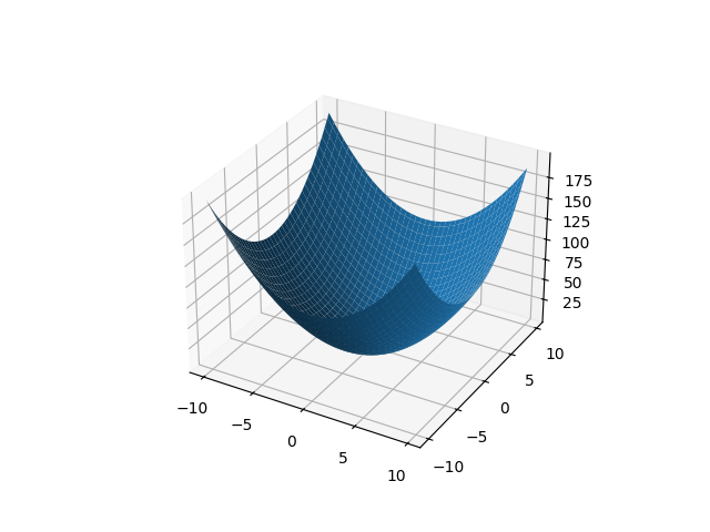
fig = plt.figure()
ax = fig.add_subplot(projection="3d")
ax.plot_surface(X, Y, Z)

plt.show()

___________________________________________________________________________

                                  GEKPLS
___________________________________________________________________________

 Problem size

      # training points.        : 20

___________________________________________________________________________

 Training

   Training ...
   Training - done. Time (sec):  0.0415080

Options

List of options

Option	Default	Acceptable values	Acceptable types	Description
print_global	True	None	[‘bool’]	Global print toggle. If False, all printing is suppressed
print_training	True	None	[‘bool’]	Whether to print training information
print_prediction	True	None	[‘bool’]	Whether to print prediction information
print_problem	True	None	[‘bool’]	Whether to print problem information
print_solver	True	None	[‘bool’]	Whether to print solver information
poly	constant	[‘constant’, ‘linear’, ‘quadratic’]	[‘str’]	Regression function type
corr	squar_exp	[‘abs_exp’, ‘squar_exp’]	[‘str’]	Correlation function type
pow_exp_power	1.9	None	[‘float’]	Power for the pow_exp kernel function (valid values in (0.0, 2.0]), This option is set automatically when corr option is squar, abs, or matern.
categorical_kernel	MixIntKernelType.CONT_RELAX	[<MixIntKernelType.CONT_RELAX: ‘CONT_RELAX’>, <MixIntKernelType.GOWER: ‘GOWER’>, <MixIntKernelType.EXP_HOMO_HSPHERE: ‘EXP_HOMO_HSPHERE’>, <MixIntKernelType.HOMO_HSPHERE: ‘HOMO_HSPHERE’>, <MixIntKernelType.COMPOUND_SYMMETRY: ‘COMPOUND_SYMMETRY’>]	None	The kernel to use for categorical inputs. Only for non continuous Kriging
hierarchical_kernel	MixHrcKernelType.ALG_KERNEL	[<MixHrcKernelType.ALG_KERNEL: ‘ALG_KERNEL’>, <MixHrcKernelType.ARC_KERNEL: ‘ARC_KERNEL’>]	None	The kernel to use for mixed hierarchical inputs. Only for non continuous Kriging
nugget	2.220446049250313e-14	None	[‘float’]	a jitter for numerical stability
theta0	[0.01]	None	[‘list’, ‘ndarray’]	Initial hyperparameters
theta_bounds	[1e-06, 20.0]	None	[‘list’, ‘ndarray’]	bounds for hyperparameters
hyper_opt	Cobyla	[‘Cobyla’]	[‘str’]	Optimiser for hyperparameters optimisation
eval_noise	False	[True, False]	[‘bool’]	noise evaluation flag
noise0	[0.0]	None	[‘list’, ‘ndarray’]	Initial noise hyperparameters
noise_bounds	[2.220446049250313e-14, 10000000000.0]	None	[‘list’, ‘ndarray’]	bounds for noise hyperparameters
use_het_noise	False	[True, False]	[‘bool’]	heteroscedastic noise evaluation flag
n_start	10	None	[‘int’]	number of optimizer runs (multistart method)
xlimits	None	None	[‘list’, ‘ndarray’]	definition of a design space of float (continuous) variables: array-like of size nx x 2 (lower, upper bounds)
design_space	None	None	[‘BaseDesignSpace’, ‘list’, ‘ndarray’]	definition of the (hierarchical) design space: use smt.utils.design_space.DesignSpace as the main API. Also accepts list of float variable bounds
random_state	41	None	[‘NoneType’, ‘int’, ‘RandomState’]	Numpy RandomState object or seed number which controls random draws for internal optim (set by default to get reproductibility)
n_comp	2	None	[‘int’]	Number of principal components
eval_n_comp	False	[True, False]	[‘bool’]	n_comp evaluation flag
eval_comp_treshold	1.0	None	[‘float’]	n_comp evaluation treshold for Wold’s R criterion
cat_kernel_comps	None	None	[‘list’]	Number of components for PLS categorical kernel
delta_x	0.0001	None	[‘int’, ‘float’]	Step used in the FOTA
extra_points	0	None	[‘int’]	Number of extra points per training point