Kriging

Kriging is an interpolating model that is a linear combination of a known function \(f_i({\bf x})\) which is added to a realization of a stochastic process \(Z({\bf x})\)

\[\hat{y} = \sum\limits_{i=1}^k\beta_if_i({\bf x})+Z({\bf x}).\]

\(Z({\bf x})\) is a realization of a stochastic process with mean zero and spatial covariance function given by

\[cov\left[Z\left({\bf x}^{(i)}\right),Z\left({\bf x}^{(j)}\right)\right] =\sigma^2R\left({\bf x}^{(i)},{\bf x}^{(j)}\right)\]

where \(\sigma^2\) is the process variance, and \(R\) is the correlation. Four types of correlation functions are available in SMT.

Exponential correlation function (Ornstein-Uhlenbeck process):

\[\prod\limits_{l=1}^{nx}\exp\left(-\theta_l\left|x_l^{(i)}-x_l^{(j)}\right|\right), \quad \forall\ \theta_l\in\mathbb{R}^+\]

Squared Exponential (Gaussian) correlation function:

\[\prod\limits_{l=1}^{nx}\exp\left(-\theta_l\left(x_l^{(i)}-x_l^{(j)}\right)^{2}\right), \quad \forall\ \theta_l\in\mathbb{R}^+\]

Exponential correlation function with a variable power:

\[\prod\limits_{l=1}^{nx}\exp\left(-\theta_l\left|x_l^{(i)}-x_l^{(j)}\right|^{p}\right), \quad \forall\ \theta_l\in\mathbb{R}^+\]

Matérn 5/2 correlation function:

\[\prod\limits_{l=1}^{nx} \left(1 + \sqrt{5}\theta_{l}\left|x_l^{(i)}-x_l^{(j)}\right| + \frac{5}{3}\theta_{l}^{2}\left(x_l^{(i)}-x_l^{(j)}\right)^{2}\right) \exp\left(-\sqrt{5}\theta_{l}\left|x_l^{(i)}-x_l^{(j)}\right|\right), \quad \forall\ \theta_l\in\mathbb{R}^+\]

Matérn 3/2 correlation function:

\[\prod\limits_{l=1}^{nx} \left(1 + \sqrt{3}\theta_{l}\left|x_l^{(i)}-x_l^{(j)}\right|\right) \exp\left(-\sqrt{3}\theta_{l}\left|x_l^{(i)}-x_l^{(j)}\right|\right), \quad \forall\ \theta_l\in\mathbb{R}^+\]

Exponential Squared Sine correlation function:

\[\prod\limits_{l=1}^{nx}\exp\left(-\theta_{l_1} \left( \sin \left( \theta_{l_2} \left( x_l^{(i)}-x_l^{(j)} \right)\right)^{2} \right) \right), \quad \forall\ \theta_l\in\mathbb{R}^+\]

These correlation functions are called by ‘abs_exp’ (exponential), ‘squar_exp’ (Gaussian), ‘matern52’,’matern32’ and ‘squar_sin_exp’ in SMT.

The deterministic term \(\sum\limits_{i=1}^k\beta_i f_i({\bf x})\) can be replaced by a constant, a linear model, or a quadratic model. These three types are available in SMT.

In the implementations, data are normalized by substracting the mean from each variable (indexed by columns in X), and then dividing the values of each variable by its standard deviation:

\[X_{\text{norm}} = \frac{X - X_{\text{mean}}}{X_{\text{std}}}\]

More details about the Kriging approach could be found in [1].

Kriging with categorical or integer variables

The goal is to be able to build a model for mixed typed variables. This algorithm has been presented by Garrido-Merchán and Hernández-Lobato in 2020 [2].

To incorporate integer (with order relation) and categorical variables (with no order), we used continuous relaxation. For integer, we add a continuous dimension with the same bounds and then we round in the prediction to the closer integer. For categorical, we add as many continuous dimensions with bounds [0,1] as possible output values for the variable and then we round in the prediction to the output dimension giving the greatest continuous prediction.

A special case is the use of the Gower distance to handle mixed integer variables (hence the gower kernel/correlation model option). See the MixedInteger Tutorial for such usage.

More details available in [2]. See also Mixed integer surrogate.

Implementation Note: Mixed variables handling is available for all Kriging models (KRG, KPLS or KPLSK) but cannot be used with derivatives computation.

[1]

Sacks, J. and Schiller, S. B. and Welch, W. J., Designs for computer experiments, Technometrics 31 (1) (1989) 41–47.

[2] (1,2)

5. 3. Garrido-Merchan and D. Hernandez-Lobato, Dealing with categorical and integer-valued variables in Bayesian Optimization with Gaussian processes, Neurocomputing 380 (2020) 20-–35.

Usage

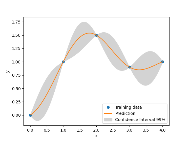
Example 1

import numpy as np
import matplotlib.pyplot as plt

from smt.surrogate_models import KRG

xt = np.array([0.0, 1.0, 2.0, 3.0, 4.0])
yt = np.array([0.0, 1.0, 1.5, 0.9, 1.0])

sm = KRG(theta0=[1e-2])
sm.set_training_values(xt, yt)
sm.train()

num = 100
x = np.linspace(0.0, 4.0, num)
y = sm.predict_values(x)
# estimated variance
s2 = sm.predict_variances(x)
# derivative according to the first variable
_dydx = sm.predict_derivatives(xt, 0)
_, axs = plt.subplots(1)

# add a plot with variance
axs.plot(xt, yt, "o")
axs.plot(x, y)
axs.fill_between(
    np.ravel(x),
    np.ravel(y - 3 * np.sqrt(s2)),
    np.ravel(y + 3 * np.sqrt(s2)),
    color="lightgrey",
)
axs.set_xlabel("x")
axs.set_ylabel("y")
axs.legend(
    ["Training data", "Prediction", "Confidence Interval 99%"],
    loc="lower right",
)

plt.show()

___________________________________________________________________________

                                  Kriging
___________________________________________________________________________

 Problem size

      # training points.        : 5

___________________________________________________________________________

 Training

   Training ...
   Training - done. Time (sec):  0.1566455
___________________________________________________________________________

 Evaluation

      # eval points. : 100

   Predicting ...
   Predicting - done. Time (sec):  0.0029492

   Prediction time/pt. (sec) :  0.0000295

___________________________________________________________________________

 Evaluation

      # eval points. : 5

   Predicting ...
   Predicting - done. Time (sec):  0.0005305

   Prediction time/pt. (sec) :  0.0001061

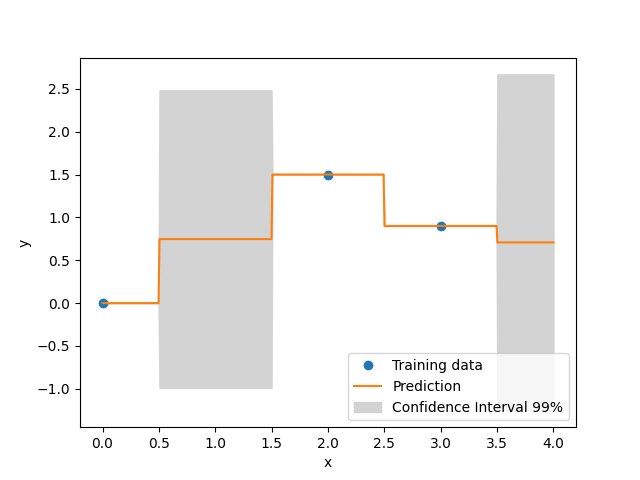
Example 2 with mixed variables

import numpy as np
import matplotlib.pyplot as plt

from smt.surrogate_models import KRG
from smt.applications.mixed_integer import MixedIntegerKrigingModel
from smt.utils.design_space import DesignSpace, IntegerVariable

xt = np.array([0.0, 2.0, 3.0])
yt = np.array([0.0, 1.5, 0.9])

design_space = DesignSpace(
    [
        IntegerVariable(0, 4),
    ]
)
sm = MixedIntegerKrigingModel(
    surrogate=KRG(design_space=design_space, theta0=[1e-2], hyper_opt="Cobyla")
)
sm.set_training_values(xt, yt)
sm.train()

num = 500
x = np.linspace(0.0, 4.0, num)
y = sm.predict_values(x)
# estimated variance
s2 = sm.predict_variances(x)

fig, axs = plt.subplots(1)
axs.plot(xt, yt, "o")
axs.plot(x, y)
axs.fill_between(
    np.ravel(x),
    np.ravel(y - 3 * np.sqrt(s2)),
    np.ravel(y + 3 * np.sqrt(s2)),
    color="lightgrey",
)
axs.set_xlabel("x")
axs.set_ylabel("y")
axs.legend(
    ["Training data", "Prediction", "Confidence Interval 99%"],
    loc="lower right",
)

plt.show()

___________________________________________________________________________

 Evaluation

      # eval points. : 500

   Predicting ...
   Predicting - done. Time (sec):  0.0096734

   Prediction time/pt. (sec) :  0.0000193

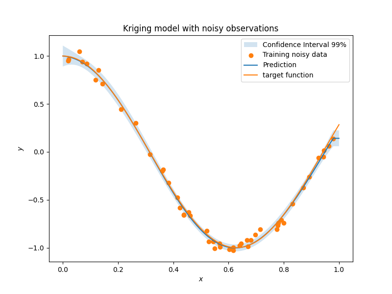
Example 3 with noisy data

import numpy as np
import matplotlib.pyplot as plt
from smt.surrogate_models import KRG

# defining the toy example
def target_fun(x):
    import numpy as np

    return np.cos(5 * x)

nobs = 50  # number of obsertvations
np.random.seed(0)  # a seed for reproducibility
xt = np.random.uniform(size=nobs)  # design points

# adding a random noise to observations
yt = target_fun(xt) + np.random.normal(scale=0.05, size=nobs)

# training the model with the option eval_noise= True
sm = KRG(eval_noise=True)
sm.set_training_values(xt, yt)
sm.train()

# predictions
x = np.linspace(0, 1, 100).reshape(-1, 1)
y = sm.predict_values(x)  # predictive mean
var = sm.predict_variances(x)  # predictive variance

# plotting predictions +- 3 std confidence intervals
plt.rcParams["figure.figsize"] = [8, 4]
plt.fill_between(
    np.ravel(x),
    np.ravel(y - 3 * np.sqrt(var)),
    np.ravel(y + 3 * np.sqrt(var)),
    alpha=0.2,
    label="Confidence Interval 99%",
)
plt.scatter(xt, yt, label="Training noisy data")
plt.plot(x, y, label="Prediction")
plt.plot(x, target_fun(x), label="target function")
plt.title("Kriging model with noisy observations")
plt.legend(loc=0)
plt.xlabel(r"$x$")
plt.ylabel(r"$y$")

___________________________________________________________________________

                                  Kriging
___________________________________________________________________________

 Problem size

      # training points.        : 50

___________________________________________________________________________

 Training

   Training ...
   Training - done. Time (sec):  0.3628881
___________________________________________________________________________

 Evaluation

      # eval points. : 100

   Predicting ...
   Predicting - done. Time (sec):  0.0112629

   Prediction time/pt. (sec) :  0.0001126

Options

List of options

Option	Default	Acceptable values	Acceptable types	Description
print_global	True	None	[‘bool’]	Global print toggle. If False, all printing is suppressed
print_training	True	None	[‘bool’]	Whether to print training information
print_prediction	True	None	[‘bool’]	Whether to print prediction information
print_problem	True	None	[‘bool’]	Whether to print problem information
print_solver	True	None	[‘bool’]	Whether to print solver information
poly	constant	[‘constant’, ‘linear’, ‘quadratic’]	[‘str’]	Regression function type
corr	squar_exp	[‘pow_exp’, ‘abs_exp’, ‘squar_exp’, ‘squar_sin_exp’, ‘matern52’, ‘matern32’]	[‘str’]	Correlation function type
pow_exp_power	1.9	None	[‘float’]	Power for the pow_exp kernel function (valid values in (0.0, 2.0]). This option is set automatically when corr option is squar, abs, or matern.
categorical_kernel	MixIntKernelType.CONT_RELAX	[<MixIntKernelType.CONT_RELAX: ‘CONT_RELAX’>, <MixIntKernelType.GOWER: ‘GOWER’>, <MixIntKernelType.EXP_HOMO_HSPHERE: ‘EXP_HOMO_HSPHERE’>, <MixIntKernelType.HOMO_HSPHERE: ‘HOMO_HSPHERE’>, <MixIntKernelType.COMPOUND_SYMMETRY: ‘COMPOUND_SYMMETRY’>]	None	The kernel to use for categorical inputs. Only for non continuous Kriging
hierarchical_kernel	MixHrcKernelType.ALG_KERNEL	[<MixHrcKernelType.ALG_KERNEL: ‘ALG_KERNEL’>, <MixHrcKernelType.ARC_KERNEL: ‘ARC_KERNEL’>]	None	The kernel to use for mixed hierarchical inputs. Only for non continuous Kriging
nugget	2.220446049250313e-14	None	[‘float’]	a jitter for numerical stability
theta0	[0.01]	None	[‘list’, ‘ndarray’]	Initial hyperparameters
theta_bounds	[1e-06, 20.0]	None	[‘list’, ‘ndarray’]	bounds for hyperparameters
hyper_opt	TNC	[‘Cobyla’, ‘TNC’]	[‘str’]	Optimiser for hyperparameters optimisation
eval_noise	False	[True, False]	[‘bool’]	noise evaluation flag
noise0	[0.0]	None	[‘list’, ‘ndarray’]	Initial noise hyperparameters
noise_bounds	[2.220446049250313e-14, 10000000000.0]	None	[‘list’, ‘ndarray’]	bounds for noise hyperparameters
use_het_noise	False	[True, False]	[‘bool’]	heteroscedastic noise evaluation flag
n_start	10	None	[‘int’]	number of optimizer runs (multistart method)
xlimits	None	None	[‘list’, ‘ndarray’]	definition of a design space of float (continuous) variables: array-like of size nx x 2 (lower, upper bounds)
design_space	None	None	[‘BaseDesignSpace’, ‘list’, ‘ndarray’]	definition of the (hierarchical) design space: use smt.utils.design_space.DesignSpace as the main API. Also accepts list of float variable bounds
random_state	41	None	[‘NoneType’, ‘int’, ‘RandomState’]	Numpy RandomState object or seed number which controls random draws for internal optim (set by default to get reproductibility)