Mixture of experts (MOE)

Mixture of experts aims at increasing the accuracy of a function approximation by replacing a single global model by a weighted sum of local models (experts). It is based on a partition of the problem domain into several subdomains via clustering algorithms followed by a local expert training on each subdomain.

A general introduction about the mixture of experts can be found in [1] and a first application with generalized linear models in [2].

SMT MOE combines surrogate models implemented in SMT to build a new surrogate model. The method is expected to improve the accuracy for functions with some of the following characteristics: heterogeneous behaviour depending on the region of the input space, flat and steep regions, first and zero order discontinuities.

The MOE method strongly relies on the Expectation-Maximization (EM) algorithm for Gaussian mixture models (GMM). With an aim of regression, the different steps are the following:

1. Clustering: the inputs are clustered together with their output values by means of parameter estimation of the joint distribution.

2. Local expert training: A local expert is then built (linear, quadratic, cubic, radial basis functions, or different forms of kriging) on each cluster

3. Recombination: all the local experts are finally combined using the Gaussian mixture model parameters found by the EM algorithm to get a global model.

When local models \(y_i\) are known, the global model would be:

\[\begin{equation}\label{e:globalMOE} \hat{y}({\bf x})=\sum_{i=1}^{K} \mathbb{P}(\kappa=i|X={\bf x}) \hat{y_i}({\bf x}) \end{equation}\]

which is the classical probability expression of mixture of experts.

In this equation, \(K\) is the number of Gaussian components, \(\mathbb{P}(\kappa=i|X= {\bf x})\), denoted by gating network, is the probability to lie in cluster \(i\) knowing that \(X = {\bf x}\) and \(\hat{y_i}\) is the local expert built on cluster \(i\).

This equation leads to two different approximation models depending on the computation of \(\mathbb{P}(\kappa=i|X={\bf x})\).

• When choosing the Gaussian laws to compute this quantity, the equation leads to a smooth model that smoothly recombine different local experts.

• If \(\mathbb{P}(\kappa=i|X= {\bf x})\) is computed as characteristic functions of clusters (being equal to 0 or 1) this leads to a discontinuous approximation model.

More details can be found in [3] and [4].

References

[1]

Jerome Friedman, Trevor Hastie, and Robert Tibshirani. The elements of statistical learning, volume 1. Springer series in statistics Springer, Berlin, 2008.

[2]

Michael I Jordan and Robert A Jacobs. Hierarchical mixtures of experts and the em algorithm. Neural computation, 6(2) :181–214, 1994.

[3]

Dimitri Bettebghor, Nathalie Bartoli, Stephane Grihon, Joseph Morlier, and Manuel Samuelides. Surrogate modeling approximation using a mixture of experts based on EM joint estimation. Structural and Multidisciplinary Optimization, 43(2) :243–259, 2011. 10.1007/s00158-010-0554-2.

[4]

Rhea P. Liem, Charles A. Mader, and Joaquim R. R. A. Martins. Surrogate models and mixtures of experts in aerodynamic performance prediction for mission analysis. Aerospace Science and Technology, 43 :126–151, 2015.

Implementation Notes

Beside the main class MOE, one can also use the MOESurrogateModel class which adapts MOE as a SurrogateModel implementing the Surrogate Model API (see Surrogate Model API).

Usage

Example 1

import numpy as np
from smt.applications import MOE
from smt.sampling_methods import FullFactorial
import matplotlib.pyplot as plt

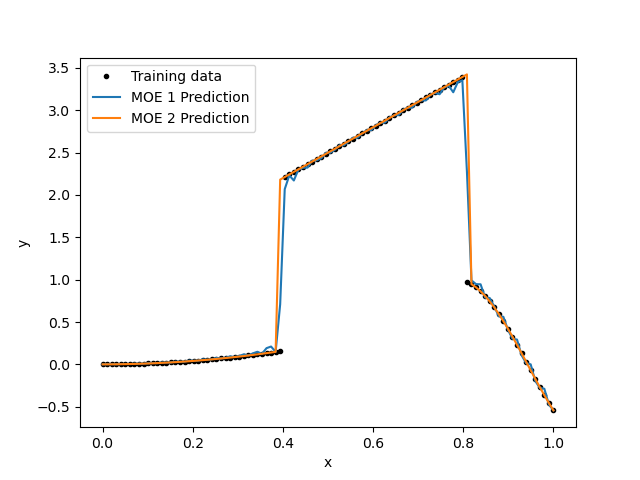
nt = 35

def function_test_1d(x):
    import numpy as np  # Note: only required by SMT doc testing toolchain

    x = np.reshape(x, (-1,))
    y = np.zeros(x.shape)
    y[x < 0.4] = x[x < 0.4] ** 2
    y[(x >= 0.4) & (x < 0.8)] = 3 * x[(x >= 0.4) & (x < 0.8)] + 1
    y[x >= 0.8] = np.sin(10 * x[x >= 0.8])
    return y.reshape((-1, 1))

x = np.linspace(0, 1, 100)
ytrue = function_test_1d(x)

# Training data
sampling = FullFactorial(xlimits=np.array([[0, 1]]), clip=True)
np.random.seed(0)
xt = sampling(nt)
yt = function_test_1d(xt)

# Mixture of experts
print("MOE Experts: ", MOE.AVAILABLE_EXPERTS)

# MOE1: Find the best surrogate model on the whole domain
moe1 = MOE(n_clusters=1)
print("MOE1 enabled experts: ", moe1.enabled_experts)
moe1.set_training_values(xt, yt)
moe1.train()
y_moe1 = moe1.predict_values(x)

# MOE2: Set nb of cluster with just KRG, LS and IDW surrogate models
moe2 = MOE(smooth_recombination=False, n_clusters=3, allow=["KRG", "LS", "IDW"])
print("MOE2 enabled experts: ", moe2.enabled_experts)
moe2.set_training_values(xt, yt)
moe2.train()
y_moe2 = moe2.predict_values(x)

fig, axs = plt.subplots(1)
axs.plot(x, ytrue, ".", color="black")
axs.plot(x, y_moe1)
axs.plot(x, y_moe2)
axs.set_xlabel("x")
axs.set_ylabel("y")
axs.legend(["Training data", "MOE 1 Prediction", "MOE 2 Prediction"])

plt.show()

MOE Experts:  ['KRG', 'KPLS', 'KPLSK', 'LS', 'QP', 'RBF', 'IDW', 'RMTB', 'RMTC']
MOE1 enabled experts:  ['KRG', 'LS', 'QP', 'KPLS', 'KPLSK', 'RBF', 'RMTC', 'RMTB', 'IDW']
Kriging 1.0248585420277574
LS 2.0995727775991893
QP 2.310722069846135
KPLS 1.0248585420277574
KPLSK 1.0248585420277574
RBF 0.7122105680266524
RMTC 0.45282839745731696
RMTB 0.35975786450312036
IDW 0.12658286305366004
Best expert = IDW
MOE2 enabled experts:  ['KRG', 'LS', 'IDW']
Kriging 7.35408919603987e-07
LS 0.03086687850659722
IDW 0.00366740075240353
Best expert = Kriging
Kriging 6.093385751526625e-08
LS 0.0
IDW 0.0018250194376276951
Best expert = LS
Kriging 3.882207838090679e-06
LS 0.07309199964574886
IDW 0.06980900375922333
Best expert = Kriging

Example 2

import numpy as np
from smt.applications import MOE
from smt.problems import LpNorm
from smt.sampling_methods import FullFactorial

import sklearn
import matplotlib.pyplot as plt
from matplotlib import colors
from mpl_toolkits.mplot3d import Axes3D

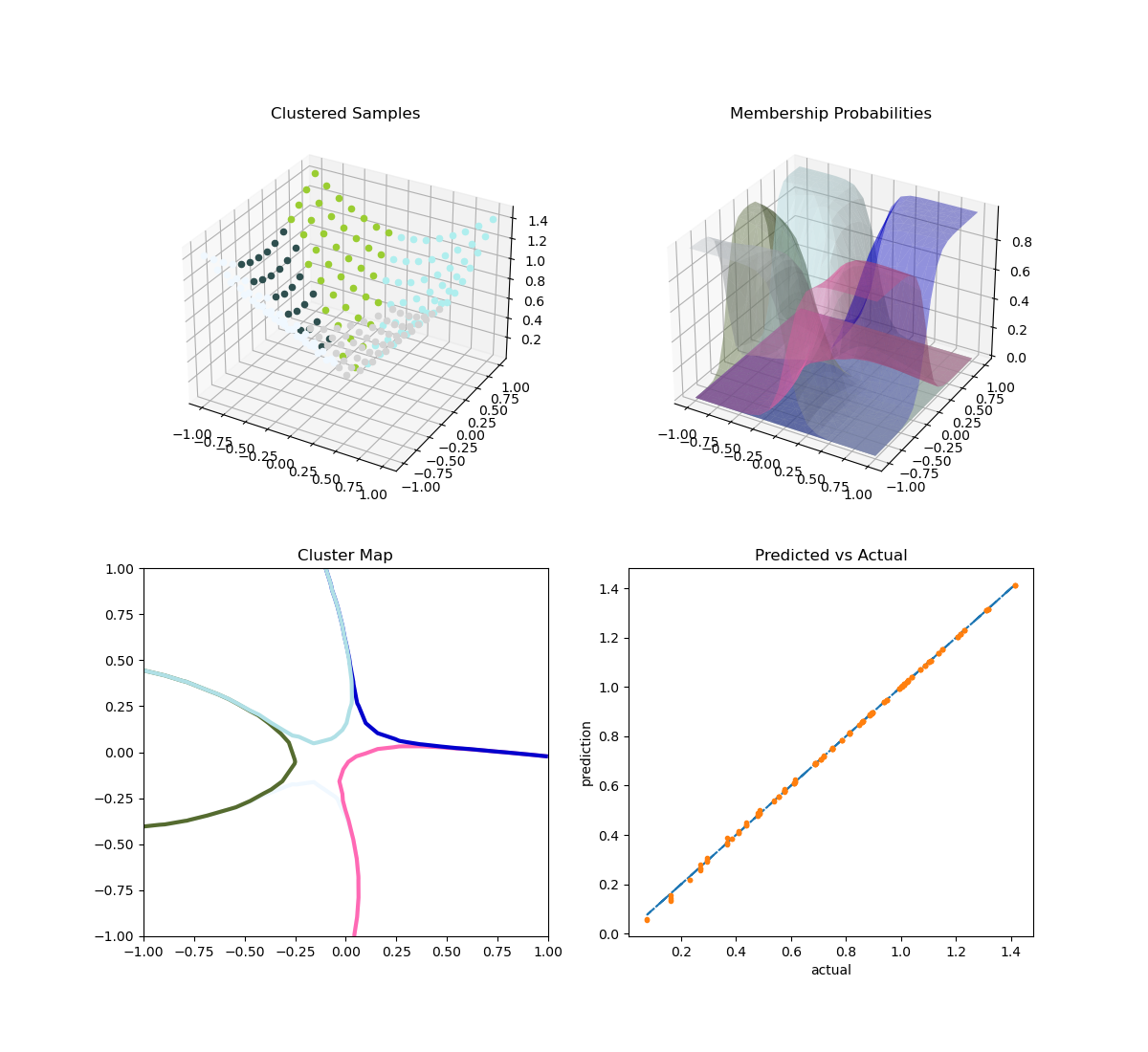
ndim = 2
nt = 200
ne = 200

# Problem: L1 norm (dimension 2)
prob = LpNorm(ndim=ndim)

# Training data
sampling = FullFactorial(xlimits=prob.xlimits, clip=True)
np.random.seed(0)
xt = sampling(nt)
yt = prob(xt)

# Mixture of experts
print("MOE Experts: ", MOE.AVAILABLE_EXPERTS)

moe = MOE(smooth_recombination=True, n_clusters=5, deny=["RMTB", "KPLSK"])
print("Enabled Experts: ", moe.enabled_experts)
moe.set_training_values(xt, yt)
moe.train()

# Validation data
np.random.seed(1)
xe = sampling(ne)
ye = prob(xe)

# Prediction
y = moe.predict_values(xe)
fig = plt.figure(1)
fig.set_size_inches(12, 11)

# Cluster display
colors_ = list(colors.cnames.items())
GMM = moe.cluster
weight = GMM.weights_
mean = GMM.means_
if sklearn.__version__ < "0.20.0":
    cov = GMM.covars_
else:
    cov = GMM.covariances_
prob_ = moe._proba_cluster(xt)
sort = np.apply_along_axis(np.argmax, 1, prob_)

xlim = prob.xlimits
x0 = np.linspace(xlim[0, 0], xlim[0, 1], 20)
x1 = np.linspace(xlim[1, 0], xlim[1, 1], 20)
xv, yv = np.meshgrid(x0, x1)
x = np.array(list(zip(xv.reshape((-1,)), yv.reshape((-1,)))))
prob = moe._proba_cluster(x)

plt.subplot(221, projection="3d")
ax = plt.gca()
for i in range(len(sort)):
    color = colors_[int(((len(colors_) - 1) / sort.max()) * sort[i])][0]
    ax.scatter(xt[i][0], xt[i][1], yt[i], c=color)
plt.title("Clustered Samples")

plt.subplot(222, projection="3d")
ax = plt.gca()
for i in range(len(weight)):
    color = colors_[int(((len(colors_) - 1) / len(weight)) * i)][0]
    ax.plot_trisurf(
        x[:, 0], x[:, 1], prob[:, i], alpha=0.4, linewidth=0, color=color
    )
plt.title("Membership Probabilities")

plt.subplot(223)
for i in range(len(weight)):
    color = colors_[int(((len(colors_) - 1) / len(weight)) * i)][0]
    plt.tricontour(x[:, 0], x[:, 1], prob[:, i], 1, colors=color, linewidths=3)
plt.title("Cluster Map")

plt.subplot(224)
plt.plot(ye, ye, "-.")
plt.plot(ye, y, ".")
plt.xlabel("actual")
plt.ylabel("prediction")
plt.title("Predicted vs Actual")

plt.show()

MOE Experts:  ['KRG', 'KPLS', 'KPLSK', 'LS', 'QP', 'RBF', 'IDW', 'RMTB', 'RMTC']
Enabled Experts:  ['KRG', 'LS', 'QP', 'KPLS', 'RBF', 'RMTC', 'IDW']
Kriging 0.0004654053099093372
LS 0.07157076020656904
QP 0.02217838851038167
KPLS 0.00042228278166402475
RBF 0.0008988900158068231
RMTC 0.027073054299467013
IDW 0.23729513276511724
Best expert = KPLS
Kriging 0.002210908084095246
LS 0.04486521104672596
QP 0.017186868491651075
KPLS 1.0368790398597236
RBF 0.0027028250420197703
RMTC 0.036342925075256924
IDW 0.25149856997477293
Best expert = Kriging
Kriging 0.0007909358332963483
LS 0.1004848526982306
QP 0.032881665708381975
KPLS 0.0007142669088972311
RBF 0.0008723419092391876
RMTC 0.026507188424772923
IDW 0.1672279524416464
Best expert = KPLS
Kriging 0.004640373019002567
LS 0.2084314251325521
QP 0.04830566919024468
KPLS 0.0016594323642259263
RBF 0.0017776802527973163
RMTC 0.02267613009449598
IDW 0.24113676800837835
Best expert = KPLS
Kriging 0.00015876585149447405
LS 0.10034642438446555
QP 0.016137577961415787
KPLS 0.00011826131245580286
RBF 0.00012095247613367939
RMTC 0.037434891675746394
IDW 0.10818152180292166
Best expert = KPLS

Options

List of options

Option	Default	Acceptable values	Acceptable types	Description
xt	None	None	[‘ndarray’]	Training inputs
yt	None	None	[‘ndarray’]	Training outputs
ct	None	None	[‘ndarray’]	Training derivative outputs used for clustering
xtest	None	None	[‘ndarray’]	Test inputs
ytest	None	None	[‘ndarray’]	Test outputs
ctest	None	None	[‘ndarray’]	Derivatives test outputs used for clustering
n_clusters	2	None	[‘int’]	Number of clusters
smooth_recombination	True	None	[‘bool’]	Continuous cluster transition
heaviside_optimization	False	None	[‘bool’]	Optimize Heaviside scaling factor when smooth recombination is used
derivatives_support	False	None	[‘bool’]	Use only experts that support derivatives prediction
variances_support	False	None	[‘bool’]	Use only experts that support variance prediction
allow	[]	None	None	Names of allowed experts to be possibly part of the mixture. Empty list corresponds to all surrogates allowed.
deny	[]	None	None	Names of forbidden experts