Proper Orthogonal Decomposition + Interpolation (PODI)¶

PODI is an application used to predict vectorial outputs. It combines Proper Orthogonal Decomposition (POD) and kriging based surrogate models to perform the estimations.

Context¶

We consider a problem in which the estimation of a vectorial output $u\in\mathbb{R}^p$ is desired. This vector depends of an input variable $\mathbf{x}=(\mathbf{x_1},\dots,\mathbf{x_N})\in\mathbb{R}^N$ representing the caracteristics of $N$ configurations of the problem. With $k \in [\![1,N]\!]$, $u(\mathbf{x_k})$ corresponds to output values at a specific configuration. It is called a snapshot.

The $N$ snapshots are gathered in a database called the snapshot matrix:

\[\begin{split}S= \begin{bmatrix} u( \mathbf{x}_1)_1 & \dots & u( \mathbf{x}_N)_1 \\ \vdots & \ddots & \vdots \\ u( \mathbf{x}_1)_p & \dots & u( \mathbf{x}_N)_p \\ \end{bmatrix} \in \mathbb{R}^{p \times N}\end{split}\]

Each column of the matrix corresponds to a snapshot output $u(\mathbf{x_k})$.

Proper Orthogonal Decomposition (POD)¶

The vectorial output $u$ is a vector of dimension $p$. Its POD is this decomposition:

\[\begin{equation}\label{e:pod} u({\mathbf x})=u_0 + \sum_{i=1}^{M} \alpha_i(\mathbf x)\phi_i \end{equation}\]

$u$ is decomposed as a sum of $M$ modes and $u_0$ corresponds to the mean value of $u$.
each mode $i$ is defined by a scalar coefficient $\alpha_i$ and a vector $\phi_{i}$ of dimension $p$.
the $\phi_i$ vectors are orthogonal and form the POD basis.

We can also define the matricial POD equation:

\[\begin{equation}\label{e:matrixPOD} S=U_0+\Phi A \end{equation}\]

where $U_0$ is composed of the $u_0$ vector on each column,

\[\begin{split}A= \begin{bmatrix} \alpha_1( \mathbf{x}_1) & \dots & \alpha_1( \mathbf{x}_N) \\ \vdots & \ddots & \vdots \\ \alpha_M( \mathbf{x}_1) & \dots & \alpha_M( \mathbf{x}_N) \\ \end{bmatrix} \text{, } \Phi= \begin{bmatrix} (\phi_1)_1 & \dots & (\phi_M)_1 \\ \vdots & \ddots & \vdots \\ (\phi_1)_p & \dots & (\phi_M)_p \\ \end{bmatrix}\end{split}\]

Singular Values Decomposition (SVD)¶

To perform the POD, the SVD of the snapshot matrix $S$ is used:

\[\begin{equation}\label{e:svd} S=U\Sigma{V}^{T} \end{equation}\]

The $(p \times p)$ $U$ and $(N \times N)$ ${V}^{T}$ matrices are orthogonal and contain the singular vectors. These vectors are the directions of maximum variance in the data and are ranked by decreasing order of importance. Each vector corresponds to a mode of $u$. The total number of available modes is limited by the number of snapshots:

\[\begin{equation}\label{e:M<=N} M \le N \end{equation}\]

The importance of each mode is represented by the diagonal values of the $(p \times N)$ $\Sigma$ matrix. They are known as the singular values $\sigma_i$ and are positive numbers ranked by decreasing value. It is then needed to filter the modes to keep those that represent most of the data structure. To do this, we use the explained variance. It represents the data variance that we keep when filtering the modes.

If $m$ modes are kept, their explained variance $EV_m$ is:

\[\begin{equation}\label{e:ev_m} EV_m=\frac{\sum_{i=1}^{m} \sigma_i}{\sum_{i=1}^{N} \sigma_i} \end{equation}\]

The number of kept modes is defined by a tolerance $\eta \in ]0,1]$ that represents the minimum variance we desire to explain during the SVD:

\[\begin{equation}\label{e:M_def} M = \min\{m \in [\![1,N]\!]: EV_m \ge \eta\} \end{equation}\]

Then, the first $M$ singular vectors of the $U$ matrix correspond to the $\phi_i$ vectors in the POD. The $\alpha_i$ coefficients of the $A$ matrix can be deduced:

\[\begin{equation}\label{e:A} A={\Phi}^{T}(S-U_0) \end{equation}\]

Use of Surrogate models¶

To compute $u$ at a new value $\mathbf{x}_*$, the values of $\alpha_i(\mathbf{x}_*)$ at each mode $i$ are needed.

To estimate them, kriging based surrogate models are used:

\[\begin{split}\mathbf{x}=(\mathbf{x}_1,\dots,\mathbf{x}_k,\dots,\mathbf{x}_N) \longrightarrow \begin{cases} \alpha_1(\mathbf{x}) \longrightarrow \text{model 1} \\ \vdots \\ \alpha_i(\mathbf{x}) \longrightarrow \text{model i} \\ \vdots \\ \alpha_M(\mathbf{x}) \longrightarrow \text{model M} \\ \end{cases}\end{split}\]

For each kept mode $i$, we use a surrogate model that is trained with the inputs $\mathbf{x}_k$ and outputs $\alpha_i(\mathbf{x}_k)$.

These models are able to compute an estimation denoted $\hat\alpha_i(\mathbf{x}_*)$. It is normally distributed:

\[\hat\alpha_i(\mathbf{x}_*) \hookrightarrow \mathcal{N}(\mu_i(\mathbf{x}_*),\sigma_i^{2}(\mathbf{x}_*))\]

The mean, variance and derivative of $u(\mathbf{x}_*)$ can be deduced:

\[\begin{split}\begin{cases} \mathbb{E}[u(\mathbf{x}_*)]=u_0+\sum_{i=1}^{M} \mu_i(\mathbf{x}_*)\phi_i \\ \mathbb{V}[u(\mathbf{x}_*)]=\sum_{i=1}^{M} \sigma_i^{2}(\mathbf{x}_*)\phi_i^{2} \\ u'(\mathbf{x}_*)=\sum_{i=1}^{M} \hat\alpha_i'(\mathbf{x}_*)\phi_i \end{cases}\end{split}\]

NB: The variance equation takes in consideration that:

the models are pairwise independent, so are the coefficients $\hat\alpha_i(\mathbf{x}_*)$.

Usage¶

import numpy as np
from smt.sampling_methods import LHS
from smt.applications import PODI
import matplotlib.pyplot as plt

light_pink = np.array((250, 233, 232)) / 255

p = 100
y = np.linspace(-1, 1, p)
n_modes_test = 10

def function_test_1d(x, y, n_modes_test, p):
    import numpy as np  # Note: only required by SMT doc testing toolchain

    def cos_coeff(i: int, x: np.ndarray):
        a = 2 * i % 2 - 1
        return a * x[:, 0] * np.cos(i * x[:, 0])

    def Legendre(i: int, y: np.ndarray):
        from scipy import special

        return special.legendre(i)(y)

    def gram_schmidt(input_array: np.ndarray) -> np.ndarray:
        """To perform the  Gram-Schmidt's algorithm."""

        basis = np.zeros_like(input_array)
        for i in range(len(input_array)):
            basis[i] = input_array[i]
            for j in range(i):
                basis[i] -= (
                    np.dot(input_array[i], basis[j])
                    / np.dot(basis[j], basis[j])
                    * basis[j]
                )
            basis[i] /= np.linalg.norm(basis[i])
        return basis

    u0 = np.zeros((p, 1))

    alpha = np.zeros((x.shape[0], n_modes_test))
    for i in range(n_modes_test):
        alpha[:, i] = cos_coeff(i, x)

    V_init = np.zeros((p, n_modes_test))
    for i in range(n_modes_test):
        V_init[:, i] = Legendre(i, y)

    V = gram_schmidt(V_init.T).T
    database = u0 + np.dot(V, alpha.T)

    return database

seed_sampling = 42
xlimits = np.array([[0, 4]])
sampling = LHS(xlimits=xlimits, random_state=seed_sampling)

nt = 40
xt = sampling(nt)

nv = 400
xv = sampling(nv)

x = np.concatenate((xt, xv))
dbfull = function_test_1d(x, y, n_modes_test, p)

# Training data
dbt = dbfull[:, :nt]

# Validation data
dbv = dbfull[:, nt:]

podi = PODI()
seed_pod = 42
podi.compute_pod(dbt, tol=0.9999, seed=seed_pod)
podi.set_training_values(xt)
podi.train()

values = podi.predict_values(xv)
variances = podi.predict_variances(xv)

# Choosing a value from the validation inputs
i = nv // 2

diff = dbv[:, i] - values[:, i]
rms_error = np.sqrt(np.mean(diff**2))
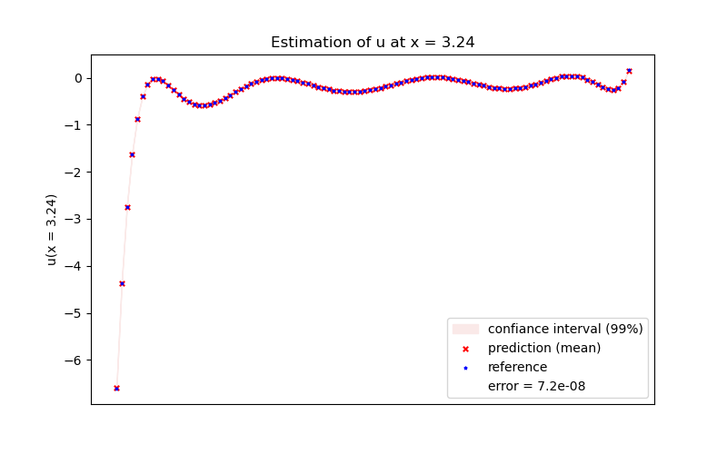
plt.figure(figsize=(8, 5))
light_pink = np.array((250, 233, 232)) / 255
plt.fill_between(
    np.ravel(y),
    np.ravel(values[:, i] - 3 * np.sqrt(variances[:, i])),
    np.ravel(values[:, i] + 3 * np.sqrt(variances[:, i])),
    color=light_pink,
    label="confiance interval (99%)",
)
plt.scatter(
    y,
    values[:, i],
    color="r",
    marker="x",
    s=15,
    alpha=1.0,
    label="prediction (mean)",
)
plt.scatter(
    y,
    dbv[:, i],
    color="b",
    marker="*",
    s=5,
    alpha=1.0,
    label="reference",
)
plt.plot([], [], color="w", label="error = " + str(round(rms_error, 9)))

ax = plt.gca()
ax.axes.xaxis.set_visible(False)

plt.ylabel("u(x = " + str(xv[i, 0])[:4] + ")")
plt.title("Estimation of u at x = " + str(xv[i, 0])[:4])
plt.legend()
plt.show()

../../_images/podi_Test_run_podi_example_1d.png

PODI class API¶

class smt.applications.podi.PODI(**kwargs)[source]¶

Class for Proper Orthogonal Decomposition and Interpolation (PODI) surrogate models based.

Examples

>>> from smt.applications import PODI
>>> sm = PODI()

Attributes:

n_modesint: Number of kept modes during the POD.
singular_vectorsnp.ndarray: Singular vectors of the POD.
singular_valuesnp.ndarray: Singular values of the POD.
interp_coefflist[SurrogateModel]: List containing the surrogate models used.

Methods

`choice_n_modes_tol`(EV_list, tol)	Static method calculating the required number of kept modes to explain at least the intended ratio of variance.
`compute_pod`(database[, tol, n_modes, seed])	Performs the POD.
`get_ev_ratio`()	Getter for the explained variance ratio with the kept modes.
`get_interp_coeff`()	Getter for the list of the interpolation surrogate models used
`get_n_modes`()	Getter for the number of modes kept during the POD.
`get_singular_values`()	Getter for the singular values from the Sigma matrix of the POD.
`get_singular_vectors`()	Getter for the singular vectors of the POD.
`predict_derivatives`(xn, kx)	Predict the dy_dx derivatives at a set of points.
`predict_values`(xn)	Predict the output values at a set of points.
`predict_variances`(xn)	Predict the variances at a set of points.
`set_interp_options`([interp_type, interp_options])	Set the options for the interpolation surrogate models used.
`set_training_values`(xt)	Set training data (values).
`train`()	Performs the training of the model.

get_singular_vectors() → ndarray[source]¶

Getter for the singular vectors of the POD. It represents the directions of maximum variance in the data.

Returns:

singular_vectorsnp.ndarray: singular vectors of the POD.

get_singular_values() → ndarray[source]¶

Getter for the singular values from the Sigma matrix of the POD.

Returns:

singular_valuesnp.ndarray: Singular values of the POD.

get_ev_ratio() → float[source]¶

Getter for the explained variance ratio with the kept modes.

Returns:

EV_ratiofloat: Explained variance ratio with the current kept modes.

get_n_modes() → int[source]¶

Getter for the number of modes kept during the POD.

Returns:

n_modesint: number of modes kept during the POD.

set_interp_options(interp_type: str = 'KRG', interp_options: list = [{}]) → None[source]¶

Set the options for the interpolation surrogate models used. Only required if a model different than KRG is used or if non-default options are desired for the models.

Parameters:

interp_typestr: Name of the type of surrogate model that will be used for the whole set. By default, the Kriging model is used (KRG).
interp_optionslist[dict]: List containing dictionnaries for the options. The k-th dictionnary corresponds to the options of the k-th interpolation model. If the options are common to all surogate models, only a single dictionnary is required in the list. The available options can be found in the documentation of the corresponding surrogate models. By default, the print_global options are set to ‘False’.

Examples

>>> interp_type = "KRG"
>>> dict1 = {'corr' : 'matern52', 'theta0' : [1e-2]}
>>> dict2 = {'poly' : 'quadratic'}
>>> interp_options = [dict1, dict2]
>>> sm.set_interp_options(interp_type, interp_options)

compute_pod(database: ndarray, tol: float = None, n_modes: int = None, seed: int = None) → None[source]¶

Performs the POD.

Parameters:

databasenp.ndarray[ny, nt]: Snapshot matrix. Each column corresponds to a snapshot.
tolfloat: Desired tolerance for the pod (if n_modes not set).
n_modesint: Desired number of kept modes for the pod (if tol not set).
seedint: seed number which controls random draws for internal optim. (optional)

Examples

>>> sm.compute_pod(database, tol = 0.99)

set_training_values(xt: ndarray) → None[source]¶

Set training data (values). If the models’ options are still not set, default values are used for the initialization.

Parameters:

xtnp.ndarray[nt, nx]: The input values for the nt training points.

train() → None[source]¶: Performs the training of the model.

get_interp_coeff() → ndarray[source]¶

Getter for the list of the interpolation surrogate models used

Returns:

interp_coeffnp.ndarray[n_modes]: List of the kriging models used for the POD coefficients.

predict_values(xn) → ndarray[source]¶

Predict the output values at a set of points.

Parameters:

xnnp.ndarray: Input values for the prediction points.

Returns:

ynnp.ndarray: Output values at the prediction points.

predict_variances(xn) → ndarray[source]¶

Predict the variances at a set of points.

Parameters:

xnnp.ndarray[nt, nx]: Input values for the prediction points.

Returns:

s2np.ndarray[nt, ny]: Variances.

predict_derivatives(xn, kx) → ndarray[source]¶

Predict the dy_dx derivatives at a set of points.

Parameters:

xnnp.ndarray[nt, nx]: Input values for the prediction points.
kxint: The 0-based index of the input variable with respect to which derivative is desired.

Returns:

dy_dxnp.ndarray[nt, ny]: Derivatives.

Proper Orthogonal Decomposition + Interpolation (PODI)¶

Context¶

Proper Orthogonal Decomposition (POD)¶

Singular Values Decomposition (SVD)¶

Use of Surrogate models¶

Usage¶

PODI class API¶

Table of Contents

Previous topic

Next topic

This Page