Variable-fidelity modeling (VFM)

VFM is a variable-fidelity modeling method which can use additive, multiplicative, or hybride bridge functions. SMT proposes only additive and multiplicative options.

In the additive method, high- and low-fidelity models, \(y_{\text{high}}({\bf x})\) and \(y_{\text{low}}({\bf x})\), are calibrated by adding the low-fidelity model to a function \(\gamma({\bf x})\), also called bridge function

\[y_\text{high}({\bf x})=y_\text{low}({\bf x}) + \gamma({\bf x})\]

The additive bridge function was developed by Lewis and Nash [1].

In the same way, the multiplicative bridge function is defined by

\[\gamma({\bf x})=\frac{y_\text{high}({\bf x})}{y_\text{low}({\bf x})}\]

However, the multiplicative bridge function may cause problems when one of the sampled values of the low-fidelity model is close to zero.

After the unknown bridge function \(\gamma\) and low-fidelity model \(y_\text{low}\) have been approximated with \(\hat{\gamma}\) and \(\hat{y}_\text{low}\), respectively, the response of the high-fidelity model is obtained

[1]

Lewis, R. M. and Nash, S. G., A multigrid approach to the optimization of systems governed by differential equations. AIAA Paper 2000-4890, 2000.

Usage

import matplotlib.pyplot as plt
import numpy as np

from smt.applications import VFM
from smt.problems import WaterFlow, WaterFlowLFidelity
from smt.sampling_methods import LHS

# Problem set up
ndim = 8
ntest = 500
ndoeLF = int(10 * ndim)
ndoeHF = int(3)
funLF = WaterFlowLFidelity(ndim=ndim)
funHF = WaterFlow(ndim=ndim)
deriv1 = True
deriv2 = True
LF_candidate = "QP"
Bridge_candidate = "KRG"
type_bridge = "Multiplicative"
optionsLF = {}
optionsB = {
    "theta0": [1e-2] * ndim,
    "print_prediction": False,
    "deriv": False,
    "hyper_opt": "Cobyla",
}

# Construct low/high fidelity data and validation points
sampling = LHS(xlimits=funLF.xlimits, criterion="m")
xLF = sampling(ndoeLF)
yLF = funLF(xLF)
if deriv1:
    dy_LF = np.zeros((ndoeLF, 1))
    for i in range(ndim):
        yd = funLF(xLF, kx=i)
        dy_LF = np.concatenate((dy_LF, yd), axis=1)

sampling = LHS(xlimits=funHF.xlimits, criterion="m")
xHF = sampling(ndoeHF)
yHF = funHF(xHF)
if deriv2:
    dy_HF = np.zeros((ndoeHF, 1))
    for i in range(ndim):
        yd = funHF(xHF, kx=i)
        dy_HF = np.concatenate((dy_HF, yd), axis=1)

xtest = sampling(ntest)
ytest = funHF(xtest)
dytest = np.zeros((ntest, ndim))
for i in range(ndim):
    dytest[:, i] = funHF(xtest, kx=i).T

# Initialize the extension VFM
M = VFM(
    type_bridge=type_bridge,
    name_model_LF=LF_candidate,
    name_model_bridge=Bridge_candidate,
    X_LF=xLF,
    y_LF=yLF,
    X_HF=xHF,
    y_HF=yHF,
    options_LF=optionsLF,
    options_bridge=optionsB,
    dy_LF=dy_LF,
    dy_HF=dy_HF,
)

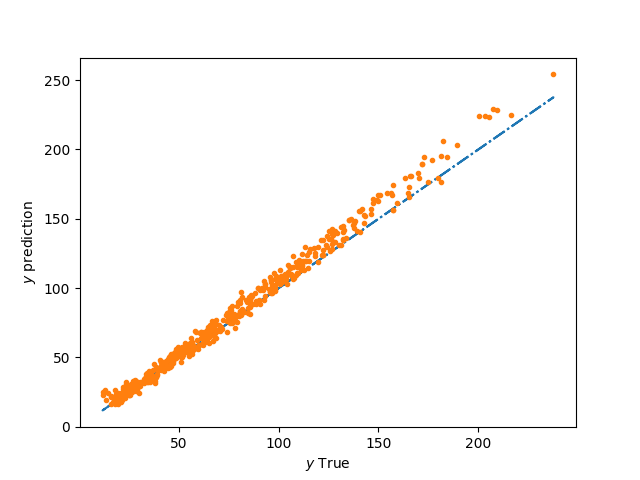
# Prediction of the validation points
y = M.predict_values(x=xtest)

plt.figure()
plt.plot(ytest, ytest, "-.")
plt.plot(ytest, y, ".")
plt.xlabel(r"$y$ True")
plt.ylabel(r"$y$ prediction")
plt.show()

___________________________________________________________________________

                                  Kriging
___________________________________________________________________________

 Problem size

      # training points.        : 3

___________________________________________________________________________

 Training

   Training ...
   Training - done. Time (sec):  0.2855706

Options

List of options

Option	Default	Acceptable values	Acceptable types	Description
name_model_LF	None	[‘KRG’, ‘LS’, ‘QP’, ‘KPLS’, ‘KPLSK’, ‘GEKPLS’, ‘RBF’, ‘RMTC’, ‘RMTB’, ‘IDW’]	[‘object’]	Name of the low-fidelity model
options_LF	{}	None	[‘dict’]	Options for the low-fidelity model
name_model_bridge	None	[‘KRG’, ‘LS’, ‘QP’, ‘KPLS’, ‘KPLSK’, ‘GEKPLS’, ‘RBF’, ‘RMTC’, ‘RMTB’, ‘IDW’]	[‘object’]	Name of the bridge model
options_bridge	{}	None	[‘dict’]	Options for the bridge model
type_bridge	Additive	[‘Additive’, ‘Multiplicative’]	[‘str’]	Bridge function type
X_LF	None	None	[‘ndarray’]	Low-fidelity inputs
y_LF	None	None	[‘ndarray’]	Low-fidelity output
X_HF	None	None	[‘ndarray’]	High-fidelity inputs
y_HF	None	None	[‘ndarray’]	High-fidelity output
dy_LF	None	None	[‘ndarray’]	Low-fidelity derivatives
dy_HF	None	None	[‘ndarray’]	High-fidelity derivatives