Radial basis functions

The radial basis function (RBF) surrogate model represents the interpolating function as a linear combination of basis functions, one for each training point. RBFs are named as such because the basis functions depend only on the distance from the prediction point to the training point for the basis function. The coefficients of the basis functions are computed during the training stage. RBFs are frequently augmented to global polynomials to capture the general trends.

The prediction equation for RBFs is

\[y = \mathbf{p}(\mathbf{x}) \mathbf{w_p} + \sum_i^{nt} \phi(\mathbf{x}, \mathbf{xt}_i) \mathbf{w_r} ,\]

where \(\mathbf{x} \in \mathbb{R}^{nx}\) is the prediction input vector, \(y \in \mathbb{R}\) is the prediction output, \(\mathbf{xt}_i \in \mathbb{R}^{nx}\) is the input vector for the \(i\) th training point, \(\mathbf{p}(\mathbf{x}) \in \mathbb{R}^{np}\) is the vector mapping the polynomial coefficients to the prediction output, \(\phi(\mathbf{x}, \mathbf{xt}_i) \in \mathbb{R}^{nt}\) is the vector mapping the radial basis function coefficients to the prediction output, \(\mathbf{w_p} \in \mathbb{R}^{np}\) is the vector of polynomial coefficients, and \(\mathbf{w_r} \in \mathbb{R}^{nt}\) is the vector of radial basis function coefficients.

The coefficients, \(\mathbf{w_p}\) and \(\mathbf{w_r}\), are computed by solving the follow linear system:

\[\begin{split}\begin{bmatrix} \phi( \mathbf{xt}_1 , \mathbf{xt}_1 ) & \dots & \phi( \mathbf{xt}_1 , \mathbf{xt}_{nt} ) & \mathbf{p}(\mathbf{xt}_1) ^ T \\ \vdots & \ddots & \vdots & \vdots \\ \phi( \mathbf{xt}_{nt} , \mathbf{xt}_1 ) & \dots & \phi( \mathbf{xt}_{nt} , \mathbf{xt}_{nt} ) & \mathbf{p}( \mathbf{xt}_{nt} ) ^ T \\ \mathbf{p}( \mathbf{xt}_1 ) & \dots & \mathbf{p}( \mathbf{xt}_{nt} ) & \mathbf{0} \\ \end{bmatrix} \begin{bmatrix} \mathbf{w_r}_1 \\ \vdots \\ \mathbf{w_r}_{nt} \\ \mathbf{w_p} \\ \end{bmatrix} = \begin{bmatrix} yt_1 \\ \vdots \\ yt_{nt} \\ 0 \\ \end{bmatrix}\end{split}\]

Only Gaussian basis functions are currently implemented. These are given by:

\[\phi( \mathbf{x}_i , \mathbf{x}_j ) = \exp \left(- \frac{|| \mathbf{x}_i - \mathbf{x}_j ||_2 ^ 2}{d_0^2} \right)\]

where \(d_0\) is a scaling parameter.

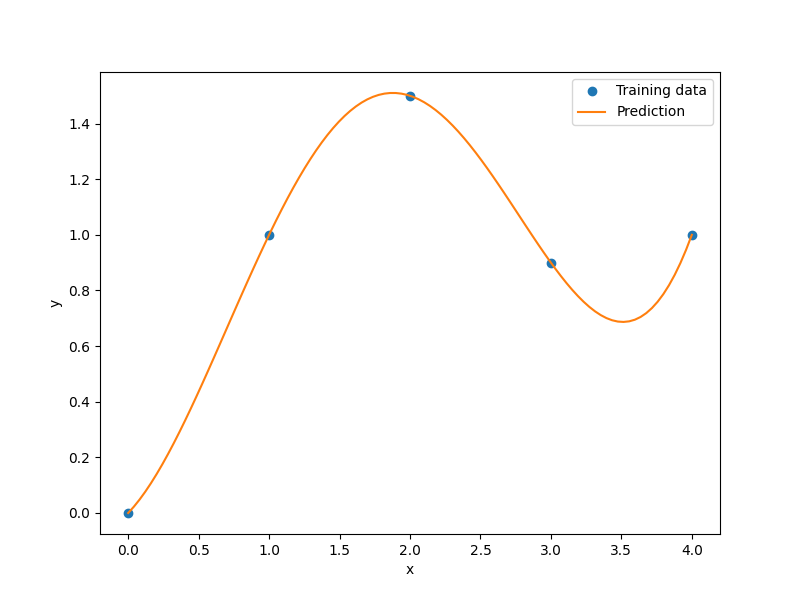
Usage

import matplotlib.pyplot as plt
import numpy as np

from smt.surrogate_models import RBF

xt = np.array([0.0, 1.0, 2.0, 3.0, 4.0])
yt = np.array([0.0, 1.0, 1.5, 0.9, 1.0])

sm = RBF(d0=5)
sm.set_training_values(xt, yt)
sm.train()

num = 100
x = np.linspace(0.0, 4.0, num)
y = sm.predict_values(x)

plt.plot(xt, yt, "o")
plt.plot(x, y)
plt.xlabel("x")
plt.ylabel("y")
plt.legend(["Training data", "Prediction"])
plt.show()

___________________________________________________________________________

                                    RBF
___________________________________________________________________________

 Problem size

      # training points.        : 5

___________________________________________________________________________

 Training

   Training ...
      Initializing linear solver ...
         Performing LU fact. (5 x 5 mtx) ...
         Performing LU fact. (5 x 5 mtx) - done. Time (sec):  0.0000000
      Initializing linear solver - done. Time (sec):  0.0000000
      Solving linear system (col. 0) ...
         Back solving (5 x 5 mtx) ...
         Back solving (5 x 5 mtx) - done. Time (sec):  0.0000000
      Solving linear system (col. 0) - done. Time (sec):  0.0000000
   Training - done. Time (sec):  0.0000000
___________________________________________________________________________

 Evaluation

      # eval points. : 100

   Predicting ...
   Predicting - done. Time (sec):  0.0000000

   Prediction time/pt. (sec) :  0.0000000

Options

List of options

Option	Default	Acceptable values	Acceptable types	Description
print_global	True	None	[‘bool’]	Global print toggle. If False, all printing is suppressed
print_training	True	None	[‘bool’]	Whether to print training information
print_prediction	True	None	[‘bool’]	Whether to print prediction information
print_problem	True	None	[‘bool’]	Whether to print problem information
print_solver	True	None	[‘bool’]	Whether to print solver information
d0	1.0	None	[‘int’, ‘float’, ‘list’, ‘ndarray’]	basis function scaling parameter in exp(-d^2 / d0^2)
poly_degree	-1	[-1, 0, 1]	[‘int’]	-1 means no global polynomial, 0 means constant, 1 means linear trend
data_dir	None	None	[‘str’]	Directory for loading / saving cached data; None means do not save or load
reg	1e-10	None	[‘int’, ‘float’]	Regularization coeff.
max_print_depth	5	None	[‘int’]	Maximum depth (level of nesting) to print operation descriptions and times