Surrogate modeling methods
SMT contains the surrogate modeling methods listed below.
Usage
import matplotlib.pyplot as plt
import numpy as np
from smt.surrogate_models import RBF
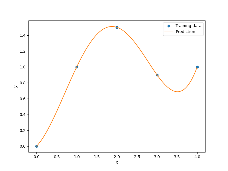
xt = np.array([0.0, 1.0, 2.0, 3.0, 4.0])
yt = np.array([0.0, 1.0, 1.5, 0.9, 1.0])
sm = RBF(d0=5)
sm.set_training_values(xt, yt)
sm.train()
num = 100
x = np.linspace(0.0, 4.0, num)
y = sm.predict_values(x)
plt.plot(xt, yt, "o")
plt.plot(x, y)
plt.xlabel("x")
plt.ylabel("y")
plt.legend(["Training data", "Prediction"])
plt.show()
___________________________________________________________________________

                                    RBF
___________________________________________________________________________

 Problem size

      # training points.        : 5

___________________________________________________________________________

 Training

   Training ...
      Initializing linear solver ...
         Performing LU fact. (5 x 5 mtx) ...
         Performing LU fact. (5 x 5 mtx) - done. Time (sec):  0.0000000
      Initializing linear solver - done. Time (sec):  0.0000000
      Solving linear system (col. 0) ...
         Back solving (5 x 5 mtx) ...
         Back solving (5 x 5 mtx) - done. Time (sec):  0.0000000
      Solving linear system (col. 0) - done. Time (sec):  0.0000000
   Training - done. Time (sec):  0.0000000
___________________________________________________________________________

 Evaluation

      # eval points. : 100

   Predicting ...
   Predicting - done. Time (sec):  0.0000000

   Prediction time/pt. (sec) :  0.0000000
SurrogateModel class API
All surrogate modeling methods implement the following API, though some of the functions in the API are not supported by all methods.
- class smt.surrogate_models.surrogate_model.SurrogateModel(**kwargs)[source]
Base class for all surrogate models.
- Attributes:
- optionsOptionsDictionary
Dictionary of options. Options values can be set on this attribute directly or they can be passed in as keyword arguments during instantiation.
- supportsdict
Dictionary containing information about what this surrogate model supports.
Methods
load(filename)Static method implemented by each surrogate model type (ie class) to load the surrogate object from a file created by using the corresponding save method
predict_derivatives(x, kx)Predict the dy_dx derivatives at a set of points.
Predict the derivatives dy_dyt at a set of points.
Predict the output values at a set of points.
predict_variance_derivatives(x, kx)Provide the derivatives of the variance of the model at a set of points.
Provide the gradient of the variance of the model at a given point (ie the derivatives wrt to all component at a unique point x)
Predict the variances at a set of points.
save(filename)Implemented by surrogate models to save the surrogate object in a file
set_training_derivatives(xt, dyt_dxt, kx[, name])Set training data (derivatives).
set_training_values(xt, yt[, name])Set training data (values).
train()Train the model
update_training_derivatives(dyt_dxt, kx[, name])Update the training data (values) at the previously set input values.
update_training_values(yt[, name])Update the training data (values) at the previously set input values.
Examples
>>> from smt.surrogate_models import RBF
>>> sm = RBF(print_training=False)
>>> sm.options['print_prediction'] = False
- __init__(**kwargs)[source]
Constructor where values of options can be passed in.
For the list of options, see the documentation for the surrogate model being used.
- Parameters:
- **kwargsnamed arguments
Set of options that can be optionally set; each option must have been declared.
Examples
>>> from smt.surrogate_models import RBF
>>> sm = RBF(print_global=False)
- set_training_values(xt: ndarray, yt: ndarray, name=None) None[source]
Set training data (values).
- Parameters:
- xtnp.ndarray[nt, nx] or np.ndarray[nt]
The input values for the nt training points.
- ytnp.ndarray[nt, ny] or np.ndarray[nt]
The output values for the nt training points.
- namestr or None
An optional label for the group of training points being set. This is only used in special situations (e.g., multi-fidelity applications).
- set_training_derivatives(xt: ndarray, dyt_dxt: ndarray, kx: int, name: str | None = None) None[source]
Set training data (derivatives).
- Parameters:
- xtnp.ndarray[nt, nx] or np.ndarray[nt]
The input values for the nt training points.
- dyt_dxtnp.ndarray[nt, ny] or np.ndarray[nt]
The derivatives values for the nt training points.
- kxint
0-based index of the derivatives being set.
- namestr or None
An optional label for the group of training points being set. This is only used in special situations (e.g., multi-fidelity applications).
- predict_values(x: ndarray) ndarray[source]
Predict the output values at a set of points.
- Parameters:
- xnp.ndarray[nt, nx] or np.ndarray[nt]
Input values for the prediction points.
- Returns:
- ynp.ndarray[nt, ny]
Output values at the prediction points.
- predict_derivatives(x: ndarray, kx: int) ndarray[source]
Predict the dy_dx derivatives at a set of points.
- Parameters:
- xnp.ndarray[nt, nx] or np.ndarray[nt]
Input values for the prediction points.
- kxint
The 0-based index of the input variable with respect to which derivatives are desired.
- Returns:
- dy_dxnp.ndarray[nt, ny]
Derivatives.
- predict_output_derivatives(x: ndarray) dict[source]
Predict the derivatives dy_dyt at a set of points.
- Parameters:
- xnp.ndarray[nt, nx] or np.ndarray[nt]
Input values for the prediction points.
- Returns:
- dy_dytdict of np.ndarray[nt, nt]
Dictionary of output derivatives. Key is None for derivatives wrt yt and kx for derivatives wrt dyt_dxt.
- predict_variances(x: ndarray) ndarray[source]
Predict the variances at a set of points.
- Parameters:
- xnp.ndarray[nt, nx] or np.ndarray[nt]
Input values for the prediction points.
- Returns:
- s2np.ndarray[nt, ny]
Variances.
- predict_variance_derivatives(x: ndarray, kx: int) ndarray[source]
Provide the derivatives of the variance of the model at a set of points.
- Parameters:
- xnp.ndarray [n_evals, dim]
Evaluation point input variable values
- kxint
The 0-based index of the input variable with respect to which derivatives are desired.
- Returns:
- derived_variance: np.ndarray
The kx-th derivatives of the variance of the kriging model
- predict_variance_gradient(x: ndarray) ndarray[source]
Provide the gradient of the variance of the model at a given point (ie the derivatives wrt to all component at a unique point x)
- Parameters:
- xnp.ndarray [1, dim] or even (dim,) vector
Evaluation point input variable values
- Returns:
- derived_variancenp.ndarray
The jacobian of the variance of the kriging model
How to save and load trained surrogate models
As of SMT 2.9, the surrogate API offers save/load methods which can be used as below.
Saving the model
The instance method save() is used to save the trained model (here KRG)
in a binary file named kriging.bin.
sm = KRG()
sm.set_training_values(xtrain, ytrain)
sm.train()

sm.save("kriging.bin ")
Loading the model
The previous model can be reloaded knowing the type of surrogate being saved (ie. KRG)
from the binary file with:
sm2 = KRG.load("kriging.bin")
ytest = sm2.predict_values(xtest)