Second-order polynomial approximation
The square polynomial model can be expressed by
\[{\bf y} = {\bf X\beta} + {\bf \epsilon},\]
where \({\bf \epsilon}\) is a vector of random errors and
\[\begin{split}{\bf X} =
\begin{bmatrix}
1&x_{1}^{(1)} & \dots&x_{nx}^{(1)} & x_{1}^{(1)}x_{2}^{(1)} & \dots & x_{nx-1}^{(1)}x_{nx}^{(1)}&{x_{1}^{(1)}}^2 & \dots&{x_{
nx}^{(1)}}^2 \\
\vdots&\vdots & \dots&\vdots & \vdots & \dots & \vdots&\vdots & \vdots\\
1&x_{1}^{(nt)} & \dots&x_{nx}^{(nt)} & x_{1}^{(nt)}x_{2}^{(nt)} & \dots & x_{nx-1}^{(nt)}x_{nx}^{(nt)}&{x_{1}^{(nt)}}^2 & \dots&{x_{
nx}^{(nt)}}^2 \\
\end{bmatrix}.\end{split}\]
The vector of estimated polynomial regression coefficients using ordinary least square estimation is
\[{\bf \beta} = {\bf X^TX}^{-1} {\bf X^Ty}.\]
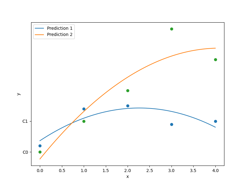
Usage
import matplotlib.pyplot as plt
import numpy as np

from smt.surrogate_models import QP

xt = np.array([[0.0, 1.0, 2.0, 3.0, 4.0]]).T
yt = np.array([[0.2, 1.4, 1.5, 0.9, 1.0], [0.0, 1.0, 2.0, 4, 3]]).T

sm = QP()
sm.set_training_values(xt, yt)
sm.train()

num = 100
x = np.linspace(0.0, 4.0, num)
y = sm.predict_values(x)

plt.plot(xt, yt[:, 0], "o", "C0")
plt.plot(x, y[:, 0], "C0", label="Prediction 1")
plt.plot(xt, yt[:, 1], "o", "C1")
plt.plot(x, y[:, 1], "C1", label="Prediction 2")
plt.xlabel("x")
plt.ylabel("y")
plt.legend()
plt.show()
___________________________________________________________________________

                                    QP
___________________________________________________________________________

 Problem size

      # training points.        : 5

___________________________________________________________________________

 Training

   Training ...
   Training - done. Time (sec):  0.0000000
___________________________________________________________________________

 Evaluation

      # eval points. : 100

   Predicting ...
   Predicting - done. Time (sec):  0.0000000

   Prediction time/pt. (sec) :  0.0000000
Options
Option |
Default |
Acceptable values |
Acceptable types |
Description |
|---|---|---|---|---|
print_global |
True |
None |
[‘bool’] |
Global print toggle. If False, all printing is suppressed |
print_training |
True |
None |
[‘bool’] |
Whether to print training information |
print_prediction |
True |
None |
[‘bool’] |
Whether to print prediction information |
print_problem |
True |
None |
[‘bool’] |
Whether to print problem information |
print_solver |
True |
None |
[‘bool’] |
Whether to print solver information |
data_dir |
None |
None |
[‘str’] |
Directory for loading / saving cached data; None means do not save or load |