Regularized minimal-energy tensor-product splines
Regularized minimal-energy tensor-product splines (RMTS) is a type of surrogate model for low-dimensional problems with large datasets and where fast prediction is desired. The underlying mathematical functions are tensor-product splines, which limits RMTS to up to 4-D problems, or 5-D problems in certain cases. On the other hand, tensor-product splines enable a very fast prediction time that does not increase with the number of training points. Unlike other methods like Kriging and radial basis functions, RMTS is not susceptible to numerical issues when there is a large number of training points or when there are points that are too close together.
The prediction equation for RMTS is
where \(\mathbf{x} \in \mathbb{R}^{nx}\) is the prediction input vector, \(y \in \mathbb{R}\) is the prediction output, \(\mathbf{w} \in \mathbb{R}^{nw}\) is the vector of spline coefficients, and \(\mathbf{F}(\mathbf{x}) \in \mathbb{R}^{nw}\) is the vector mapping the spline coefficients to the prediction output.
RMTS computes the coefficients of the splines, \(\mathbf{w}\), by solving an energy minimization problem subject to the conditions that the splines pass through the training points. This is formulated as an unconstrained optimization problem where the objective function consists of a term containing the second derivatives of the splines, another term representing the approximation error for the training points, and another term for regularization:
where \(\mathbf{xt}_i \in \mathbb{R}^{nx}\) is the input vector for the \(i\) th training point, \(yt_i \in \mathbb{R}\) is the output value for the \(i\) th training point, \(\mathbf{H} \in \mathbb{R}^{nw \times nw}\) is the matrix containing the second derivatives, \(\mathbf{F}(\mathbf{xt}_i) \in \mathbb{R}^{nw}\) is the vector mapping the spline coefficients to the \(i\) th training output, and \(\alpha\) and \(\beta\) are regularization coefficients.
In problems with a large number of training points relative to the number of spline coefficients,
the energy minimization term is not necessary;
this term can be zero-ed by setting the energy_weight option to zero.
In problems with a small dataset, the energy minimization is necessary.
When the true function has high curvature, the energy minimization can be counterproductive
in the regions of high curvature.
This can be addressed by increasing the quadratic approximation term to one of higher order,
and using Newton’s method to solve the nonlinear system that results.
The nonlinear formulation is given by
where \(p\) is the order given by the approx_order option.
The number of Newton iterations can be specified via the nonlinear_maxiter option.
RMTS is implemented in SMT with two choices of splines:
1. B-splines (RMTB): RMTB uses B-splines with a uniform knot vector in each dimension. The number of B-spline control points and the B-spline order in each dimension are options that trade off efficiency and precision of the interpolant.
2. Cubic Hermite splines (RMTC): RMTC divides the domain into tensor-product cubic elements. For adjacent elements, the values and derivatives are continuous. The number of elements in each dimension is an option that trades off efficiency and precision.
In general, RMTB is the better choice when training time is the most important, while RMTC is the better choice when accuracy of the interpolant is the most important.
More details of these methods are given in [1].
Specially with regard to the implementation, the above functions to minimize are multiplied by \(\alpha\)
which does not change the minimum result.
Then the energy_weight and regularization_weight controlling options used below are respectively defined
as \(\alpha'=\alpha\) and \(\beta'=\alpha\beta\). See the section 3.5 - Summary and implementation in [1] for further details.
Usage (RMTB)
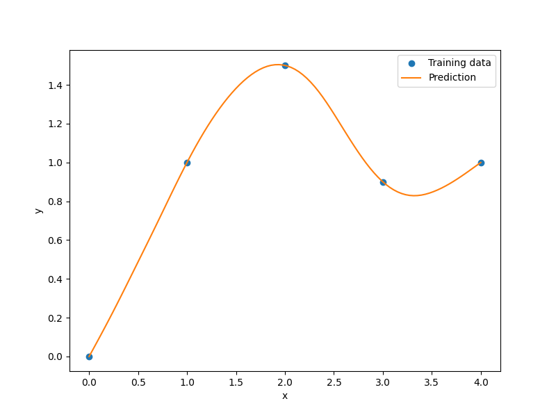
import matplotlib.pyplot as plt
import numpy as np

from smt.surrogate_models import RMTB

xt = np.array([0.0, 1.0, 2.0, 3.0, 4.0])
yt = np.array([0.0, 1.0, 1.5, 0.9, 1.0])

xlimits = np.array([[0.0, 4.0]])

sm = RMTB(
    xlimits=xlimits,
    order=4,
    num_ctrl_pts=20,
    energy_weight=1e-15,
    regularization_weight=0.0,
)
sm.set_training_values(xt, yt)
sm.train()

num = 100
x = np.linspace(0.0, 4.0, num)
y = sm.predict_values(x)

plt.plot(xt, yt, "o")
plt.plot(x, y)
plt.xlabel("x")
plt.ylabel("y")
plt.legend(["Training data", "Prediction"])
plt.show()
___________________________________________________________________________

                                   RMTB
___________________________________________________________________________

 Problem size

      # training points.        : 5

___________________________________________________________________________

 Training

   Training ...
      Pre-computing matrices ...
         Computing dof2coeff ...
         Computing dof2coeff - done. Time (sec):  0.0000000
         Initializing Hessian ...
         Initializing Hessian - done. Time (sec):  0.0000000
         Computing energy terms ...
         Computing energy terms - done. Time (sec):  0.0005453
         Computing approximation terms ...
         Computing approximation terms - done. Time (sec):  0.0000000
      Pre-computing matrices - done. Time (sec):  0.0005453
      Solving for degrees of freedom ...
         Solving initial startup problem (n=20) ...
            Solving for output 0 ...
               Iteration (num., iy, grad. norm, func.) :   0   0 1.549745600e+00 2.530000000e+00
               Iteration (num., iy, grad. norm, func.) :   0   0 1.462445337e-15 4.462575191e-16
            Solving for output 0 - done. Time (sec):  0.0000000
         Solving initial startup problem (n=20) - done. Time (sec):  0.0000000
         Solving nonlinear problem (n=20) ...
            Solving for output 0 ...
               Iteration (num., iy, grad. norm, func.) :   0   0 1.535878390e-15 4.462575191e-16
            Solving for output 0 - done. Time (sec):  0.0000000
         Solving nonlinear problem (n=20) - done. Time (sec):  0.0000000
      Solving for degrees of freedom - done. Time (sec):  0.0000000
   Training - done. Time (sec):  0.0100670
___________________________________________________________________________

 Evaluation

      # eval points. : 100

   Predicting ...
   Predicting - done. Time (sec):  0.0000000

   Prediction time/pt. (sec) :  0.0000000
Usage (RMTC)
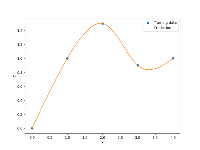
import matplotlib.pyplot as plt
import numpy as np

from smt.surrogate_models import RMTC

xt = np.array([0.0, 1.0, 2.0, 3.0, 4.0])
yt = np.array([0.0, 1.0, 1.5, 0.9, 1.0])

xlimits = np.array([[0.0, 4.0]])

sm = RMTC(
    xlimits=xlimits,
    num_elements=6,
    energy_weight=1e-15,
    regularization_weight=0.0,
)
sm.set_training_values(xt, yt)
sm.train()

num = 100
x = np.linspace(0.0, 4.0, num)
y = sm.predict_values(x)

plt.plot(xt, yt, "o")
plt.plot(x, y)
plt.xlabel("x")
plt.ylabel("y")
plt.legend(["Training data", "Prediction"])
plt.show()
___________________________________________________________________________

                                   RMTC
___________________________________________________________________________

 Problem size

      # training points.        : 5

___________________________________________________________________________

 Training

   Training ...
      Pre-computing matrices ...
         Computing dof2coeff ...
         Computing dof2coeff - done. Time (sec):  0.0050485
         Initializing Hessian ...
         Initializing Hessian - done. Time (sec):  0.0000000
         Computing energy terms ...
         Computing energy terms - done. Time (sec):  0.0000000
         Computing approximation terms ...
         Computing approximation terms - done. Time (sec):  0.0000000
      Pre-computing matrices - done. Time (sec):  0.0050485
      Solving for degrees of freedom ...
         Solving initial startup problem (n=14) ...
            Solving for output 0 ...
               Iteration (num., iy, grad. norm, func.) :   0   0 2.093143569e+00 2.530000000e+00
               Iteration (num., iy, grad. norm, func.) :   0   0 9.683718704e-16 4.386716851e-16
            Solving for output 0 - done. Time (sec):  0.0000000
         Solving initial startup problem (n=14) - done. Time (sec):  0.0000000
         Solving nonlinear problem (n=14) ...
            Solving for output 0 ...
               Iteration (num., iy, grad. norm, func.) :   0   0 1.754310197e-15 4.386716851e-16
            Solving for output 0 - done. Time (sec):  0.0000000
         Solving nonlinear problem (n=14) - done. Time (sec):  0.0000000
      Solving for degrees of freedom - done. Time (sec):  0.0000000
   Training - done. Time (sec):  0.0050485
___________________________________________________________________________

 Evaluation

      # eval points. : 100

   Predicting ...
   Predicting - done. Time (sec):  0.0000000

   Prediction time/pt. (sec) :  0.0000000
Options (RMTB)
Option |
Default |
Acceptable values |
Acceptable types |
Description |
|---|---|---|---|---|
print_global |
True |
None |
[‘bool’] |
Global print toggle. If False, all printing is suppressed |
print_training |
True |
None |
[‘bool’] |
Whether to print training information |
print_prediction |
True |
None |
[‘bool’] |
Whether to print prediction information |
print_problem |
True |
None |
[‘bool’] |
Whether to print problem information |
print_solver |
True |
None |
[‘bool’] |
Whether to print solver information |
xlimits |
None |
None |
[‘ndarray’] |
Lower/upper bounds in each dimension - ndarray [nx, 2] |
smoothness |
1.0 |
None |
[‘Integral’, ‘float’, ‘tuple’, ‘list’, ‘ndarray’] |
Smoothness parameter in each dimension - length nx. None implies uniform |
regularization_weight |
1e-14 |
None |
[‘Integral’, ‘float’] |
Weight of the term penalizing the norm of the spline coefficients. This is useful as an alternative to energy minimization when energy minimization makes the training time too long. |
energy_weight |
0.0001 |
None |
[‘Integral’, ‘float’] |
The weight of the energy minimization terms |
extrapolate |
False |
None |
[‘bool’] |
Whether to perform linear extrapolation for external evaluation points |
min_energy |
True |
None |
[‘bool’] |
Whether to perform energy minimization |
approx_order |
4 |
None |
[‘Integral’] |
Exponent in the approximation term |
solver |
krylov |
[‘krylov-dense’, ‘dense-lu’, ‘dense-chol’, ‘lu’, ‘ilu’, ‘krylov’, ‘krylov-lu’, ‘krylov-mg’, ‘gs’, ‘jacobi’, ‘mg’, ‘null’] |
[‘LinearSolver’] |
Linear solver |
derivative_solver |
krylov |
[‘krylov-dense’, ‘dense-lu’, ‘dense-chol’, ‘lu’, ‘ilu’, ‘krylov’, ‘krylov-lu’, ‘krylov-mg’, ‘gs’, ‘jacobi’, ‘mg’, ‘null’] |
[‘LinearSolver’] |
Linear solver used for computing output derivatives (dy_dyt) |
grad_weight |
0.5 |
None |
[‘Integral’, ‘float’] |
Weight on gradient training data |
solver_tolerance |
1e-12 |
None |
[‘Integral’, ‘float’] |
Convergence tolerance for the nonlinear solver |
nonlinear_maxiter |
10 |
None |
[‘Integral’] |
Maximum number of nonlinear solver iterations |
line_search |
backtracking |
[‘backtracking’, ‘bracketed’, ‘quadratic’, ‘cubic’, ‘null’] |
[‘LineSearch’] |
Line search algorithm |
save_energy_terms |
False |
None |
[‘bool’] |
Whether to cache energy terms in the data_dir directory |
data_dir |
None |
[None] |
[‘str’] |
Directory for loading / saving cached data; None means do not save or load |
max_print_depth |
5 |
None |
[‘Integral’] |
Maximum depth (level of nesting) to print operation descriptions and times |
order |
3 |
None |
[‘Integral’, ‘tuple’, ‘list’, ‘ndarray’] |
B-spline order in each dimension - length [nx] |
num_ctrl_pts |
15 |
None |
[‘Integral’, ‘tuple’, ‘list’, ‘ndarray’] |
# B-spline control points in each dimension - length [nx] |
Options (RMTC)
Option |
Default |
Acceptable values |
Acceptable types |
Description |
|---|---|---|---|---|
print_global |
True |
None |
[‘bool’] |
Global print toggle. If False, all printing is suppressed |
print_training |
True |
None |
[‘bool’] |
Whether to print training information |
print_prediction |
True |
None |
[‘bool’] |
Whether to print prediction information |
print_problem |
True |
None |
[‘bool’] |
Whether to print problem information |
print_solver |
True |
None |
[‘bool’] |
Whether to print solver information |
xlimits |
None |
None |
[‘ndarray’] |
Lower/upper bounds in each dimension - ndarray [nx, 2] |
smoothness |
1.0 |
None |
[‘Integral’, ‘float’, ‘tuple’, ‘list’, ‘ndarray’] |
Smoothness parameter in each dimension - length nx. None implies uniform |
regularization_weight |
1e-14 |
None |
[‘Integral’, ‘float’] |
Weight of the term penalizing the norm of the spline coefficients. This is useful as an alternative to energy minimization when energy minimization makes the training time too long. |
energy_weight |
0.0001 |
None |
[‘Integral’, ‘float’] |
The weight of the energy minimization terms |
extrapolate |
False |
None |
[‘bool’] |
Whether to perform linear extrapolation for external evaluation points |
min_energy |
True |
None |
[‘bool’] |
Whether to perform energy minimization |
approx_order |
4 |
None |
[‘Integral’] |
Exponent in the approximation term |
solver |
krylov |
[‘krylov-dense’, ‘dense-lu’, ‘dense-chol’, ‘lu’, ‘ilu’, ‘krylov’, ‘krylov-lu’, ‘krylov-mg’, ‘gs’, ‘jacobi’, ‘mg’, ‘null’] |
[‘LinearSolver’] |
Linear solver |
derivative_solver |
krylov |
[‘krylov-dense’, ‘dense-lu’, ‘dense-chol’, ‘lu’, ‘ilu’, ‘krylov’, ‘krylov-lu’, ‘krylov-mg’, ‘gs’, ‘jacobi’, ‘mg’, ‘null’] |
[‘LinearSolver’] |
Linear solver used for computing output derivatives (dy_dyt) |
grad_weight |
0.5 |
None |
[‘Integral’, ‘float’] |
Weight on gradient training data |
solver_tolerance |
1e-12 |
None |
[‘Integral’, ‘float’] |
Convergence tolerance for the nonlinear solver |
nonlinear_maxiter |
10 |
None |
[‘Integral’] |
Maximum number of nonlinear solver iterations |
line_search |
backtracking |
[‘backtracking’, ‘bracketed’, ‘quadratic’, ‘cubic’, ‘null’] |
[‘LineSearch’] |
Line search algorithm |
save_energy_terms |
False |
None |
[‘bool’] |
Whether to cache energy terms in the data_dir directory |
data_dir |
None |
[None] |
[‘str’] |
Directory for loading / saving cached data; None means do not save or load |
max_print_depth |
5 |
None |
[‘Integral’] |
Maximum depth (level of nesting) to print operation descriptions and times |
num_elements |
4 |
None |
[‘Integral’, ‘list’, ‘ndarray’] |
# elements in each dimension - ndarray [nx] |