Mixed integer surrogate

To use a surrogate with mixed integer constraints, the user instantiates a MixedIntegerSurrogateModel with the given surrogate. The MixedIntegerSurrogateModel implements the SurrogateModel interface and decorates the given surrogate while respecting integer and categorical types. They are various surrogate models implemented that are described below.

For Kriging models, several methods to construct the mixed categorical correlation kernel are implemented. As a consequence, the user can instantiate a MixedIntegerKrigingModel with the given kernel for Kriging. Currently, 4 methods (CR, GD, EHH and HH) are implemented that are described hereafter.

Mixed Integer Surrogate with Continuous Relaxation (CR)

For categorical variables, as many x features are added as there are levels for the variables. These new dimensions have [0, 1] bounds and the max of these feature float values will correspond to the choice of one the enum value: this is the so-called “one-hot encoding”. For instance, for a categorical variable (one feature of x) with three levels [“blue”, “red”, “green”], 3 continuous float features x0, x1, x2 are created. Thereafter, the value max(x0, x1, x2), for instance, x1, will give “red” as the value for the original categorical feature. Details can be found in [1] .

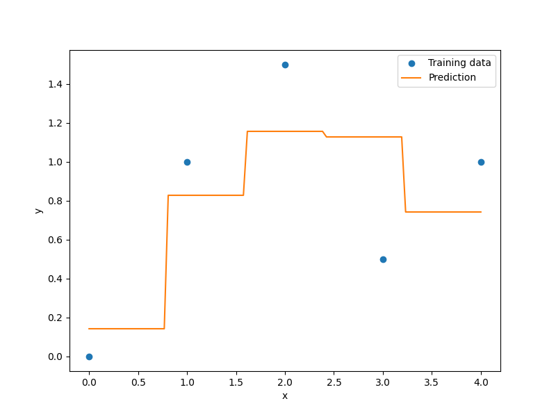
Example of mixed integer Polynomial (QP) surrogate

import numpy as np
import matplotlib.pyplot as plt

from smt.surrogate_models import QP
from smt.applications.mixed_integer import MixedIntegerSurrogateModel
from smt.utils.design_space import DesignSpace, IntegerVariable

xt = np.array([0.0, 1.0, 2.0, 3.0, 4.0])
yt = np.array([0.0, 1.0, 1.5, 0.5, 1.0])

# Specify the design space using the DesignSpace
# class and various available variable types
design_space = DesignSpace(
    [
        IntegerVariable(0, 4),
    ]
)
sm = MixedIntegerSurrogateModel(design_space=design_space, surrogate=QP())
sm.set_training_values(xt, yt)
sm.train()

num = 100
x = np.linspace(0.0, 4.0, num)
y = sm.predict_values(x)

plt.plot(xt, yt, "o")
plt.plot(x, y)
plt.xlabel("x")
plt.ylabel("y")
plt.legend(["Training data", "Prediction"])
plt.show()

___________________________________________________________________________

 Evaluation

      # eval points. : 100

   Predicting ...
   Predicting - done. Time (sec):  0.0000150

   Prediction time/pt. (sec) :  0.0000002

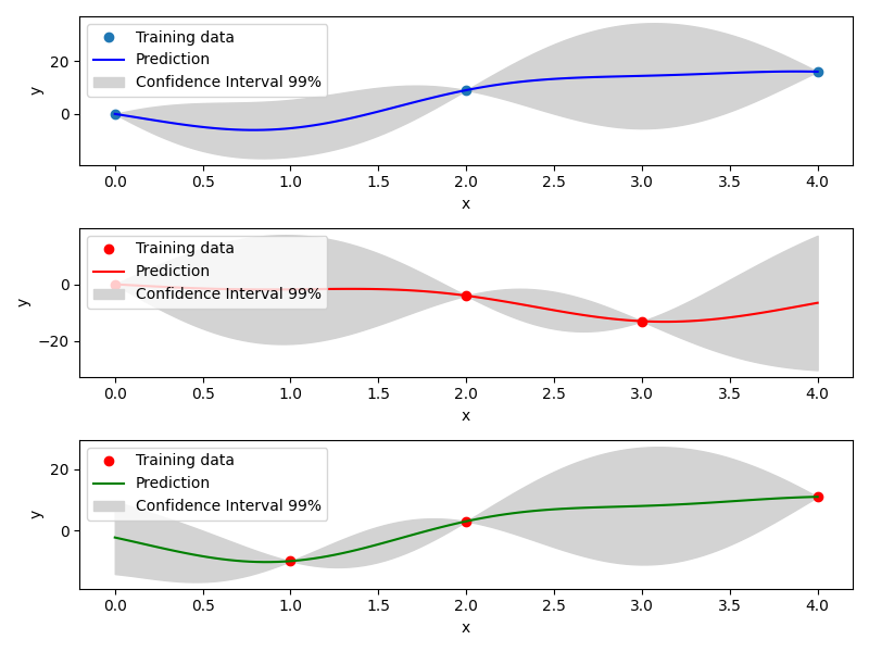
Mixed Integer Kriging with Gower Distance (GD)

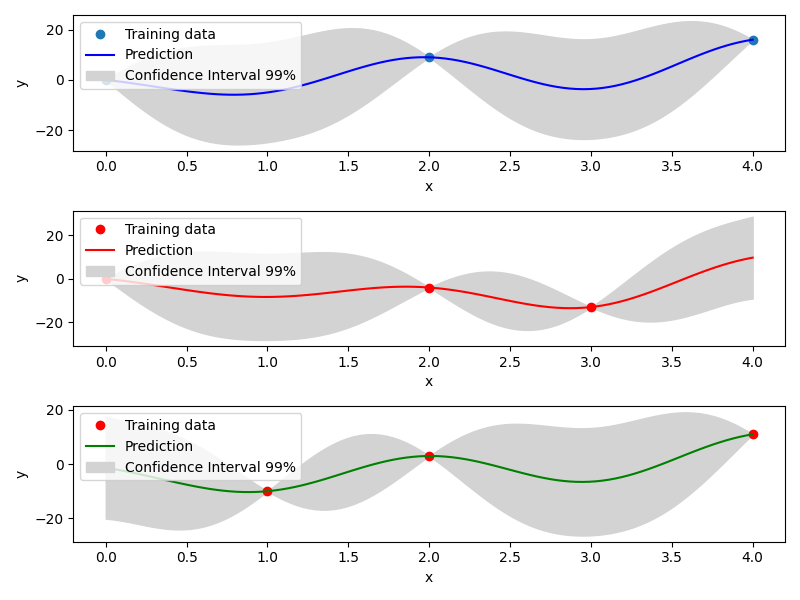
Another implemented method to tackle mixed integer with Kriging is using a basic mixed integer kernel based on the Gower distance between two points. When constructing the correlation kernel, the distance is redefined as \(\Delta= \Delta_{cont} + \Delta_{cat}\), with \(\Delta_{cont}\) the continuous distance as usual and \(\Delta_ {cat}\) the categorical distance defined as the number of categorical variables that differs from one point to another.

For example, the Gower Distance between [1,'red', 'medium'] and [1.2,'red', 'large'] is \(\Delta= 0.2+ (0\) 'red' \(=\) 'red' \(+ 1\) 'medium' \(\neq\) 'large' ) \(=1.2\). With this distance, a mixed integer kernel can be build. Details can be found in [1] .

Example of mixed integer Gower Distance model

import numpy as np
import matplotlib.pyplot as plt

from smt.surrogate_models import KRG, MixIntKernelType
from smt.applications.mixed_integer import (
    MixedIntegerKrigingModel,
)
from smt.utils.design_space import (
    DesignSpace,
    CategoricalVariable,
    FloatVariable,
)

xt1 = np.array([[0, 0.0], [0, 2.0], [0, 4.0]])
xt2 = np.array([[1, 0.0], [1, 2.0], [1, 3.0]])
xt3 = np.array([[2, 1.0], [2, 2.0], [2, 4.0]])

xt = np.concatenate((xt1, xt2, xt3), axis=0)
xt[:, 1] = xt[:, 1].astype(np.float64)
yt1 = np.array([0.0, 9.0, 16.0])
yt2 = np.array([0.0, -4, -13.0])
yt3 = np.array([-10, 3, 11.0])
yt = np.concatenate((yt1, yt2, yt3), axis=0)

design_space = DesignSpace(
    [
        CategoricalVariable(["Blue", "Red", "Green"]),
        FloatVariable(0, 4),
    ]
)

# Surrogate
sm = MixedIntegerKrigingModel(
    surrogate=KRG(
        design_space=design_space,
        categorical_kernel=MixIntKernelType.GOWER,
        theta0=[1e-1],
        corr="squar_exp",
        n_start=20,
    ),
)
sm.set_training_values(xt, yt)
sm.train()

# DOE for validation
n = 100
x_cat1 = []
x_cat2 = []
x_cat3 = []

for i in range(n):
    x_cat1.append(0)
    x_cat2.append(1)
    x_cat3.append(2)

x_cont = np.linspace(0.0, 4.0, n)
x1 = np.concatenate(
    (np.asarray(x_cat1).reshape(-1, 1), x_cont.reshape(-1, 1)), axis=1
)
x2 = np.concatenate(
    (np.asarray(x_cat2).reshape(-1, 1), x_cont.reshape(-1, 1)), axis=1
)
x3 = np.concatenate(
    (np.asarray(x_cat3).reshape(-1, 1), x_cont.reshape(-1, 1)), axis=1
)

y1 = sm.predict_values(x1)
y2 = sm.predict_values(x2)
y3 = sm.predict_values(x3)

# estimated variance
s2_1 = sm.predict_variances(x1)
s2_2 = sm.predict_variances(x2)
s2_3 = sm.predict_variances(x3)

fig, axs = plt.subplots(3, figsize=(8, 6))

axs[0].plot(xt1[:, 1].astype(np.float64), yt1, "o", linestyle="None")
axs[0].plot(x_cont, y1, color="Blue")
axs[0].fill_between(
    np.ravel(x_cont),
    np.ravel(y1 - 3 * np.sqrt(s2_1)),
    np.ravel(y1 + 3 * np.sqrt(s2_1)),
    color="lightgrey",
)
axs[0].set_xlabel("x")
axs[0].set_ylabel("y")
axs[0].legend(
    ["Training data", "Prediction", "Confidence Interval 99%"],
    loc="upper left",
    bbox_to_anchor=[0, 1],
)
axs[1].plot(
    xt2[:, 1].astype(np.float64), yt2, marker="o", color="r", linestyle="None"
)
axs[1].plot(x_cont, y2, color="Red")
axs[1].fill_between(
    np.ravel(x_cont),
    np.ravel(y2 - 3 * np.sqrt(s2_2)),
    np.ravel(y2 + 3 * np.sqrt(s2_2)),
    color="lightgrey",
)
axs[1].set_xlabel("x")
axs[1].set_ylabel("y")
axs[1].legend(
    ["Training data", "Prediction", "Confidence Interval 99%"],
    loc="upper left",
    bbox_to_anchor=[0, 1],
)
axs[2].plot(
    xt3[:, 1].astype(np.float64), yt3, marker="o", color="r", linestyle="None"
)
axs[2].plot(x_cont, y3, color="Green")
axs[2].fill_between(
    np.ravel(x_cont),
    np.ravel(y3 - 3 * np.sqrt(s2_3)),
    np.ravel(y3 + 3 * np.sqrt(s2_3)),
    color="lightgrey",
)
axs[2].set_xlabel("x")
axs[2].set_ylabel("y")
axs[2].legend(
    ["Training data", "Prediction", "Confidence Interval 99%"],
    loc="upper left",
    bbox_to_anchor=[0, 1],
)
plt.tight_layout()
plt.show()

___________________________________________________________________________

 Evaluation

      # eval points. : 100

   Predicting ...
   Predicting - done. Time (sec):  0.0029371

   Prediction time/pt. (sec) :  0.0000294

___________________________________________________________________________

 Evaluation

      # eval points. : 100

   Predicting ...
   Predicting - done. Time (sec):  0.0028622

   Prediction time/pt. (sec) :  0.0000286

___________________________________________________________________________

 Evaluation

      # eval points. : 100

   Predicting ...
   Predicting - done. Time (sec):  0.0028448

   Prediction time/pt. (sec) :  0.0000284

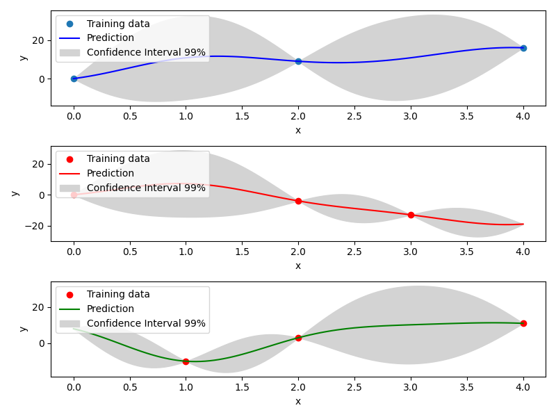
Mixed Integer Kriging with Compound Symmetry (CS)

Compound Symmetry is similar to Gower Distance but allow to model negative correlations. Details can be found in [2] .

Example of mixed integer Compound Symmetry model

import numpy as np
import matplotlib.pyplot as plt

from smt.surrogate_models import KRG, MixIntKernelType
from smt.applications.mixed_integer import (
    MixedIntegerKrigingModel,
)
from smt.utils.design_space import (
    DesignSpace,
    CategoricalVariable,
    FloatVariable,
)

xt1 = np.array([[0, 0.0], [0, 2.0], [0, 4.0]])
xt2 = np.array([[1, 0.0], [1, 2.0], [1, 3.0]])
xt3 = np.array([[2, 1.0], [2, 2.0], [2, 4.0]])

xt = np.concatenate((xt1, xt2, xt3), axis=0)
xt[:, 1] = xt[:, 1].astype(np.float64)
yt1 = np.array([0.0, 9.0, 16.0])
yt2 = np.array([0.0, -4, -13.0])
yt3 = np.array([-10, 3, 11.0])
yt = np.concatenate((yt1, yt2, yt3), axis=0)

design_space = DesignSpace(
    [
        CategoricalVariable(["Blue", "Red", "Green"]),
        FloatVariable(0, 4),
    ]
)

# Surrogate
sm = MixedIntegerKrigingModel(
    surrogate=KRG(
        design_space=design_space,
        categorical_kernel=MixIntKernelType.COMPOUND_SYMMETRY,
        theta0=[1e-1],
        corr="squar_exp",
        n_start=20,
    ),
)
sm.set_training_values(xt, yt)
sm.train()

# DOE for validation
n = 100
x_cat1 = []
x_cat2 = []
x_cat3 = []

for i in range(n):
    x_cat1.append(0)
    x_cat2.append(1)
    x_cat3.append(2)

x_cont = np.linspace(0.0, 4.0, n)
x1 = np.concatenate(
    (np.asarray(x_cat1).reshape(-1, 1), x_cont.reshape(-1, 1)), axis=1
)
x2 = np.concatenate(
    (np.asarray(x_cat2).reshape(-1, 1), x_cont.reshape(-1, 1)), axis=1
)
x3 = np.concatenate(
    (np.asarray(x_cat3).reshape(-1, 1), x_cont.reshape(-1, 1)), axis=1
)

y1 = sm.predict_values(x1)
y2 = sm.predict_values(x2)
y3 = sm.predict_values(x3)

# estimated variance
s2_1 = sm.predict_variances(x1)
s2_2 = sm.predict_variances(x2)
s2_3 = sm.predict_variances(x3)

fig, axs = plt.subplots(3, figsize=(8, 6))

axs[0].plot(xt1[:, 1].astype(np.float64), yt1, "o", linestyle="None")
axs[0].plot(x_cont, y1, color="Blue")
axs[0].fill_between(
    np.ravel(x_cont),
    np.ravel(y1 - 3 * np.sqrt(s2_1)),
    np.ravel(y1 + 3 * np.sqrt(s2_1)),
    color="lightgrey",
)
axs[0].set_xlabel("x")
axs[0].set_ylabel("y")
axs[0].legend(
    ["Training data", "Prediction", "Confidence Interval 99%"],
    loc="upper left",
    bbox_to_anchor=[0, 1],
)
axs[1].plot(
    xt2[:, 1].astype(np.float64), yt2, marker="o", color="r", linestyle="None"
)
axs[1].plot(x_cont, y2, color="Red")
axs[1].fill_between(
    np.ravel(x_cont),
    np.ravel(y2 - 3 * np.sqrt(s2_2)),
    np.ravel(y2 + 3 * np.sqrt(s2_2)),
    color="lightgrey",
)
axs[1].set_xlabel("x")
axs[1].set_ylabel("y")
axs[1].legend(
    ["Training data", "Prediction", "Confidence Interval 99%"],
    loc="upper left",
    bbox_to_anchor=[0, 1],
)
axs[2].plot(
    xt3[:, 1].astype(np.float64), yt3, marker="o", color="r", linestyle="None"
)
axs[2].plot(x_cont, y3, color="Green")
axs[2].fill_between(
    np.ravel(x_cont),
    np.ravel(y3 - 3 * np.sqrt(s2_3)),
    np.ravel(y3 + 3 * np.sqrt(s2_3)),
    color="lightgrey",
)
axs[2].set_xlabel("x")
axs[2].set_ylabel("y")
axs[2].legend(
    ["Training data", "Prediction", "Confidence Interval 99%"],
    loc="upper left",
    bbox_to_anchor=[0, 1],
)
plt.tight_layout()
plt.show()

exception :  4-th leading minor of the array is not positive definite
[ 3.28121902e+01 -1.19061651e+01 -1.19062304e+01  7.34202209e-04
 -3.09582545e-04 -2.19341599e-04  3.49847394e-09 -1.67389467e-09
 -7.15698170e-10]
exception :  4-th leading minor of the array is not positive definite
[ 9.09297095e+00 -4.69851668e-02 -4.69502417e-02  9.74106925e-04
 -5.62905232e-06 -4.04511718e-06  2.47447277e-08 -1.26347080e-10
 -6.20962350e-11]
___________________________________________________________________________

 Evaluation

      # eval points. : 100

   Predicting ...
   Predicting - done. Time (sec):  0.0033650

   Prediction time/pt. (sec) :  0.0000337

___________________________________________________________________________

 Evaluation

      # eval points. : 100

   Predicting ...
   Predicting - done. Time (sec):  0.0033152

   Prediction time/pt. (sec) :  0.0000332

___________________________________________________________________________

 Evaluation

      # eval points. : 100

   Predicting ...
   Predicting - done. Time (sec):  0.0032670

   Prediction time/pt. (sec) :  0.0000327

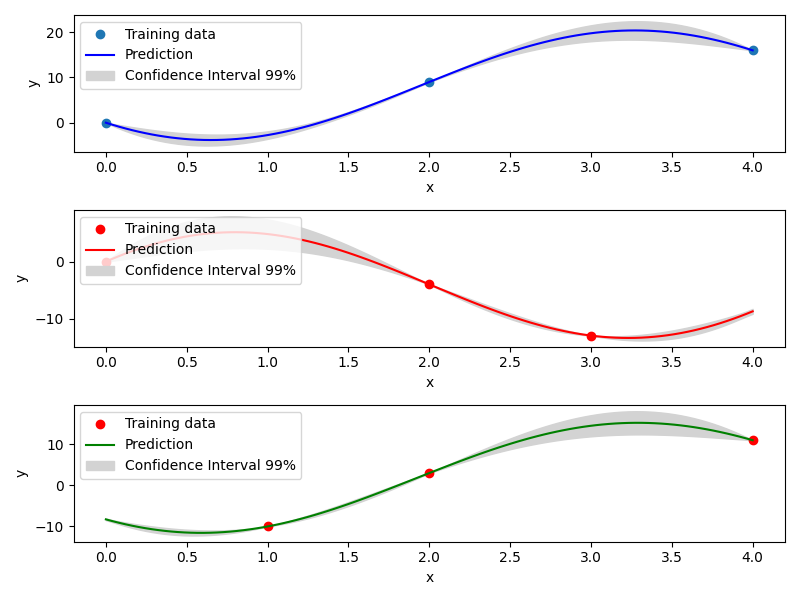
Mixed Integer Kriging with Homoscedastic Hypersphere (HH)

This surrogate model assumes that the correlation kernel between the levels of a given variable is a symmetric positive definite matrix. The latter matrix is estimated through an hypersphere parametrization depending on several hyperparameters. To finish with, the data correlation matrix is build as the product of the correlation matrices over the various variables. Details can be found in [1] . Note that this model is the only one to consider negative correlations between levels (“blue” can be correlated negatively to “red”).

Example of mixed integer Homoscedastic Hypersphere model

import numpy as np
import matplotlib.pyplot as plt

from smt.surrogate_models import KRG, MixIntKernelType
from smt.applications.mixed_integer import MixedIntegerKrigingModel
from smt.utils.design_space import (
    DesignSpace,
    CategoricalVariable,
    FloatVariable,
)

xt1 = np.array([[0, 0.0], [0, 2.0], [0, 4.0]])
xt2 = np.array([[1, 0.0], [1, 2.0], [1, 3.0]])
xt3 = np.array([[2, 1.0], [2, 2.0], [2, 4.0]])

xt = np.concatenate((xt1, xt2, xt3), axis=0)
xt[:, 1] = xt[:, 1].astype(np.float64)
yt1 = np.array([0.0, 9.0, 16.0])
yt2 = np.array([0.0, -4, -13.0])
yt3 = np.array([-10, 3, 11.0])
yt = np.concatenate((yt1, yt2, yt3), axis=0)

design_space = DesignSpace(
    [
        CategoricalVariable(["Blue", "Red", "Green"]),
        FloatVariable(0, 4),
    ]
)

# Surrogate
sm = MixedIntegerKrigingModel(
    surrogate=KRG(
        design_space=design_space,
        categorical_kernel=MixIntKernelType.HOMO_HSPHERE,
        theta0=[1e-1],
        corr="squar_exp",
        n_start=20,
    ),
)
sm.set_training_values(xt, yt)
sm.train()

# DOE for validation
n = 100
x_cat1 = []
x_cat2 = []
x_cat3 = []

for i in range(n):
    x_cat1.append(0)
    x_cat2.append(1)
    x_cat3.append(2)

x_cont = np.linspace(0.0, 4.0, n)
x1 = np.concatenate(
    (np.asarray(x_cat1).reshape(-1, 1), x_cont.reshape(-1, 1)), axis=1
)
x2 = np.concatenate(
    (np.asarray(x_cat2).reshape(-1, 1), x_cont.reshape(-1, 1)), axis=1
)
x3 = np.concatenate(
    (np.asarray(x_cat3).reshape(-1, 1), x_cont.reshape(-1, 1)), axis=1
)

y1 = sm.predict_values(x1)
y2 = sm.predict_values(x2)
y3 = sm.predict_values(x3)

# estimated variance
s2_1 = sm.predict_variances(x1)
s2_2 = sm.predict_variances(x2)
s2_3 = sm.predict_variances(x3)

fig, axs = plt.subplots(3, figsize=(8, 6))

axs[0].plot(xt1[:, 1].astype(np.float64), yt1, "o", linestyle="None")
axs[0].plot(x_cont, y1, color="Blue")
axs[0].fill_between(
    np.ravel(x_cont),
    np.ravel(y1 - 3 * np.sqrt(s2_1)),
    np.ravel(y1 + 3 * np.sqrt(s2_1)),
    color="lightgrey",
)
axs[0].set_xlabel("x")
axs[0].set_ylabel("y")
axs[0].legend(
    ["Training data", "Prediction", "Confidence Interval 99%"],
    loc="upper left",
    bbox_to_anchor=[0, 1],
)
axs[1].plot(
    xt2[:, 1].astype(np.float64), yt2, marker="o", color="r", linestyle="None"
)
axs[1].plot(x_cont, y2, color="Red")
axs[1].fill_between(
    np.ravel(x_cont),
    np.ravel(y2 - 3 * np.sqrt(s2_2)),
    np.ravel(y2 + 3 * np.sqrt(s2_2)),
    color="lightgrey",
)
axs[1].set_xlabel("x")
axs[1].set_ylabel("y")
axs[1].legend(
    ["Training data", "Prediction", "Confidence Interval 99%"],
    loc="upper left",
    bbox_to_anchor=[0, 1],
)
axs[2].plot(
    xt3[:, 1].astype(np.float64), yt3, marker="o", color="r", linestyle="None"
)
axs[2].plot(x_cont, y3, color="Green")
axs[2].fill_between(
    np.ravel(x_cont),
    np.ravel(y3 - 3 * np.sqrt(s2_3)),
    np.ravel(y3 + 3 * np.sqrt(s2_3)),
    color="lightgrey",
)
axs[2].set_xlabel("x")
axs[2].set_ylabel("y")
axs[2].legend(
    ["Training data", "Prediction", "Confidence Interval 99%"],
    loc="upper left",
    bbox_to_anchor=[0, 1],
)
plt.tight_layout()
plt.show()

___________________________________________________________________________

 Evaluation

      # eval points. : 100

   Predicting ...
   Predicting - done. Time (sec):  0.0033951

   Prediction time/pt. (sec) :  0.0000340

___________________________________________________________________________

 Evaluation

      # eval points. : 100

   Predicting ...
   Predicting - done. Time (sec):  0.0033388

   Prediction time/pt. (sec) :  0.0000334

___________________________________________________________________________

 Evaluation

      # eval points. : 100

   Predicting ...
   Predicting - done. Time (sec):  0.0033410

   Prediction time/pt. (sec) :  0.0000334

Mixed Integer Kriging with Exponential Homoscedastic Hypersphere (EHH)

This surrogate model also considers that the correlation kernel between the levels of a given variable is a symmetric positive definite matrix. The latter matrix is estimated through an hypersphere parametrization depending on several hyperparameters. Thereafter, an exponential kernel is applied to the matrix. To finish with, the data correlation matrix is build as the product of the correlation matrices over the various variables. Therefore, this model could not model negative correlation and only works with absolute exponential and Gaussian kernels. Details can be found in [1] .

Example of mixed integer Exponential Homoscedastic Hypersphere model

import numpy as np
import matplotlib.pyplot as plt

from smt.surrogate_models import KRG, MixIntKernelType
from smt.applications.mixed_integer import MixedIntegerKrigingModel
from smt.utils.design_space import (
    DesignSpace,
    CategoricalVariable,
    FloatVariable,
)

xt1 = np.array([[0, 0.0], [0, 2.0], [0, 4.0]])
xt2 = np.array([[1, 0.0], [1, 2.0], [1, 3.0]])
xt3 = np.array([[2, 1.0], [2, 2.0], [2, 4.0]])

xt = np.concatenate((xt1, xt2, xt3), axis=0)
xt[:, 1] = xt[:, 1].astype(np.float64)
yt1 = np.array([0.0, 9.0, 16.0])
yt2 = np.array([0.0, -4, -13.0])
yt3 = np.array([-10, 3, 11.0])
yt = np.concatenate((yt1, yt2, yt3), axis=0)

design_space = DesignSpace(
    [
        CategoricalVariable(["Blue", "Red", "Green"]),
        FloatVariable(0, 4),
    ]
)

# Surrogate
sm = MixedIntegerKrigingModel(
    surrogate=KRG(
        design_space=design_space,
        theta0=[1e-1],
        corr="squar_exp",
        n_start=20,
        categorical_kernel=MixIntKernelType.EXP_HOMO_HSPHERE,
    ),
)
sm.set_training_values(xt, yt)
sm.train()

# DOE for validation
n = 100
x_cat1 = []
x_cat2 = []
x_cat3 = []

for i in range(n):
    x_cat1.append(0)
    x_cat2.append(1)
    x_cat3.append(2)

x_cont = np.linspace(0.0, 4.0, n)
x1 = np.concatenate(
    (np.asarray(x_cat1).reshape(-1, 1), x_cont.reshape(-1, 1)), axis=1
)
x2 = np.concatenate(
    (np.asarray(x_cat2).reshape(-1, 1), x_cont.reshape(-1, 1)), axis=1
)
x3 = np.concatenate(
    (np.asarray(x_cat3).reshape(-1, 1), x_cont.reshape(-1, 1)), axis=1
)

y1 = sm.predict_values(x1)
y2 = sm.predict_values(x2)
y3 = sm.predict_values(x3)

# estimated variance
s2_1 = sm.predict_variances(x1)
s2_2 = sm.predict_variances(x2)
s2_3 = sm.predict_variances(x3)

fig, axs = plt.subplots(3, figsize=(8, 6))

axs[0].plot(xt1[:, 1].astype(np.float64), yt1, "o", linestyle="None")
axs[0].plot(x_cont, y1, color="Blue")
axs[0].fill_between(
    np.ravel(x_cont),
    np.ravel(y1 - 3 * np.sqrt(s2_1)),
    np.ravel(y1 + 3 * np.sqrt(s2_1)),
    color="lightgrey",
)
axs[0].set_xlabel("x")
axs[0].set_ylabel("y")
axs[0].legend(
    ["Training data", "Prediction", "Confidence Interval 99%"],
    loc="upper left",
    bbox_to_anchor=[0, 1],
)
axs[1].plot(
    xt2[:, 1].astype(np.float64), yt2, marker="o", color="r", linestyle="None"
)
axs[1].plot(x_cont, y2, color="Red")
axs[1].fill_between(
    np.ravel(x_cont),
    np.ravel(y2 - 3 * np.sqrt(s2_2)),
    np.ravel(y2 + 3 * np.sqrt(s2_2)),
    color="lightgrey",
)
axs[1].set_xlabel("x")
axs[1].set_ylabel("y")
axs[1].legend(
    ["Training data", "Prediction", "Confidence Interval 99%"],
    loc="upper left",
    bbox_to_anchor=[0, 1],
)
axs[2].plot(
    xt3[:, 1].astype(np.float64), yt3, marker="o", color="r", linestyle="None"
)
axs[2].plot(x_cont, y3, color="Green")
axs[2].fill_between(
    np.ravel(x_cont),
    np.ravel(y3 - 3 * np.sqrt(s2_3)),
    np.ravel(y3 + 3 * np.sqrt(s2_3)),
    color="lightgrey",
)
axs[2].set_xlabel("x")
axs[2].set_ylabel("y")
axs[2].legend(
    ["Training data", "Prediction", "Confidence Interval 99%"],
    loc="upper left",
    bbox_to_anchor=[0, 1],
)
plt.tight_layout()
plt.show()

___________________________________________________________________________

 Evaluation

      # eval points. : 100

   Predicting ...
   Predicting - done. Time (sec):  0.0034671

   Prediction time/pt. (sec) :  0.0000347

___________________________________________________________________________

 Evaluation

      # eval points. : 100

   Predicting ...
   Predicting - done. Time (sec):  0.0033689

   Prediction time/pt. (sec) :  0.0000337

___________________________________________________________________________

 Evaluation

      # eval points. : 100

   Predicting ...
   Predicting - done. Time (sec):  0.0033631

   Prediction time/pt. (sec) :  0.0000336

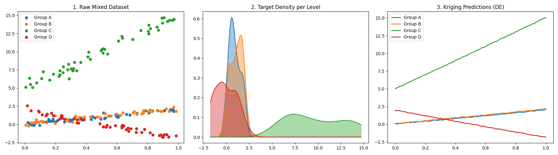
Mixed Integer Kriging with hierarchical variables

The DesignSpace class can be used to model design variable hierarchy: conditionally active design variables and value constraints. A MixedIntegerKrigingModel with both Hierarchical and Mixed-categorical variables can be build using this. Two kernels for hierarchical variables are available, namely Arc-Kernel and Alg-Kernel. More details are given in the usage section.

Example of mixed integer Kriging with hierarchical variables

import numpy as np
from smt.utils.design_space import (
    DesignSpace,
    CategoricalVariable,
    IntegerVariable,
    FloatVariable,
)
from smt.applications.mixed_integer import (
    MixedIntegerKrigingModel,
    MixedIntegerSamplingMethod,
)
from smt.surrogate_models import MixIntKernelType, MixHrcKernelType, KRG
from smt.sampling_methods import LHS

def f_hv(X):
    import numpy as np

    def H(x1, x2, x3, x4, z3, z4, x5, cos_term):
        import numpy as np

        h = (
            53.3108
            + 0.184901 * x1
            - 5.02914 * x1**3 * 10 ** (-6)
            + 7.72522 * x1**z3 * 10 ** (-8)
            - 0.0870775 * x2
            - 0.106959 * x3
            + 7.98772 * x3**z4 * 10 ** (-6)
            + 0.00242482 * x4
            + 1.32851 * x4**3 * 10 ** (-6)
            - 0.00146393 * x1 * x2
            - 0.00301588 * x1 * x3
            - 0.00272291 * x1 * x4
            + 0.0017004 * x2 * x3
            + 0.0038428 * x2 * x4
            - 0.000198969 * x3 * x4
            + 1.86025 * x1 * x2 * x3 * 10 ** (-5)
            - 1.88719 * x1 * x2 * x4 * 10 ** (-6)
            + 2.50923 * x1 * x3 * x4 * 10 ** (-5)
            - 5.62199 * x2 * x3 * x4 * 10 ** (-5)
        )
        if cos_term:
            h += 5.0 * np.cos(2.0 * np.pi * (x5 / 100.0)) - 2.0
        return h

    def f1(x1, x2, z1, z2, z3, z4, x5, cos_term):
        c1 = z2 == 0
        c2 = z2 == 1
        c3 = z2 == 2

        c4 = z3 == 0
        c5 = z3 == 1
        c6 = z3 == 2

        y = (
            c4
            * (
                c1 * H(x1, x2, 20, 20, z3, z4, x5, cos_term)
                + c2 * H(x1, x2, 50, 20, z3, z4, x5, cos_term)
                + c3 * H(x1, x2, 80, 20, z3, z4, x5, cos_term)
            )
            + c5
            * (
                c1 * H(x1, x2, 20, 50, z3, z4, x5, cos_term)
                + c2 * H(x1, x2, 50, 50, z3, z4, x5, cos_term)
                + c3 * H(x1, x2, 80, 50, z3, z4, x5, cos_term)
            )
            + c6
            * (
                c1 * H(x1, x2, 20, 80, z3, z4, x5, cos_term)
                + c2 * H(x1, x2, 50, 80, z3, z4, x5, cos_term)
                + c3 * H(x1, x2, 80, 80, z3, z4, x5, cos_term)
            )
        )
        return y

    def f2(x1, x2, x3, z2, z3, z4, x5, cos_term):
        c1 = z2 == 0
        c2 = z2 == 1
        c3 = z2 == 2

        y = (
            c1 * H(x1, x2, x3, 20, z3, z4, x5, cos_term)
            + c2 * H(x1, x2, x3, 50, z3, z4, x5, cos_term)
            + c3 * H(x1, x2, x3, 80, z3, z4, x5, cos_term)
        )
        return y

    def f3(x1, x2, x4, z1, z3, z4, x5, cos_term):
        c1 = z1 == 0
        c2 = z1 == 1
        c3 = z1 == 2

        y = (
            c1 * H(x1, x2, 20, x4, z3, z4, x5, cos_term)
            + c2 * H(x1, x2, 50, x4, z3, z4, x5, cos_term)
            + c3 * H(x1, x2, 80, x4, z3, z4, x5, cos_term)
        )
        return y

    y = []
    for x in X:
        if x[0] == 0:
            y.append(
                f1(x[2], x[3], x[7], x[8], x[9], x[10], x[6], cos_term=x[1])
            )
        elif x[0] == 1:
            y.append(
                f2(x[2], x[3], x[4], x[8], x[9], x[10], x[6], cos_term=x[1])
            )
        elif x[0] == 2:
            y.append(
                f3(x[2], x[3], x[5], x[7], x[9], x[10], x[6], cos_term=x[1])
            )
        elif x[0] == 3:
            y.append(
                H(x[2], x[3], x[4], x[5], x[9], x[10], x[6], cos_term=x[1])
            )
    return np.array(y)

design_space = DesignSpace(
    [
        CategoricalVariable(values=[0, 1, 2, 3]),  # meta
        IntegerVariable(0, 1),  # x1
        FloatVariable(0, 100),  # x2
        FloatVariable(0, 100),
        FloatVariable(0, 100),
        FloatVariable(0, 100),
        FloatVariable(0, 100),
        IntegerVariable(0, 2),  # x7
        IntegerVariable(0, 2),
        IntegerVariable(0, 2),
        IntegerVariable(0, 2),
    ]
)

# x4 is acting if meta == 1, 3
design_space.declare_decreed_var(decreed_var=4, meta_var=0, meta_value=[1, 3])
# x5 is acting if meta == 2, 3
design_space.declare_decreed_var(decreed_var=5, meta_var=0, meta_value=[2, 3])
# x7 is acting if meta == 0, 2
design_space.declare_decreed_var(decreed_var=7, meta_var=0, meta_value=[0, 2])
# x8 is acting if meta == 0, 1
design_space.declare_decreed_var(decreed_var=8, meta_var=0, meta_value=[0, 1])

# Sample from the design spaces, correctly considering hierarchy
n_doe = 15
design_space.seed = 42
samp = MixedIntegerSamplingMethod(
    LHS, design_space, criterion="ese", random_state=design_space.seed
)
Xt, Xt_is_acting = samp(n_doe, return_is_acting=True)

Yt = f_hv(Xt)

sm = MixedIntegerKrigingModel(
    surrogate=KRG(
        design_space=design_space,
        categorical_kernel=MixIntKernelType.HOMO_HSPHERE,
        hierarchical_kernel=MixHrcKernelType.ALG_KERNEL,  # ALG or ARC
        theta0=[1e-2],
        corr="abs_exp",
        n_start=5,
    ),
)
sm.set_training_values(Xt, Yt, is_acting=Xt_is_acting)
sm.train()
y_s = sm.predict_values(Xt)[:, 0]
_pred_RMSE = np.linalg.norm(y_s - Yt) / len(Yt)

y_sv = sm.predict_variances(Xt)[:, 0]
_var_RMSE = np.linalg.norm(y_sv) / len(Yt)

___________________________________________________________________________

 Evaluation

      # eval points. : 15

   Predicting ...
   Predicting - done. Time (sec):  0.0029151

   Prediction time/pt. (sec) :  0.0001943

References

[1] (1,2,3,4)

Saves, P. and Diouane, Y. and Bartoli, N. and Lefebvre, T. and Morlier, J. (2022). A general square exponential kernel to handle mixed-categorical variables for Gaussian process. AIAA Aviation 2022 Forum.

[2]

Pelamatti, J. “Mixed-variable Bayesian optimization: application to aerospace system design”, PhD thesis, Université de Lille, Lille, 2020.