Sparse Gaussian Process (SGP)

Although the versatility of Gaussian Process regression models for learning complex data, their computational complexity, which is \(\mathcal{O}(N^3)\) with \(N\) the number of training points, prevent their use to large datasets. This complexity results from the inversion of the covariance matrix \(\mathbf{K}\). We must also highlight that the memory cost of GPR models is \(\mathcal{O}(N^2)\), mainly due to the storage of the covariance matrix itself.

To address these limitations, sparse GPs approximation methods have emerged as efficient alternatives. Sparse GPs consider a set of inducing points to approximate the posterior Gaussian distribution with a low-rank representation, while the variational inference provides a framework for approximating the posterior distribution directly. Thus, these methods enable accurate modeling of large datasets while preserving computational efficiency (typically \(\mathcal{O}(NM^2)\) time and \(\mathcal{O}(NM)\) memory for some chosen \(M<N\)).

See [1] for a detailed information and discussion on several approximation methods benefits and drawbacks.

Implementation

In SMT the methods: Fully Independent Training Conditional (FITC) method and the Variational Free Energy (VFE) approximation are implemented inspired from inference methods developed in the GPy project [2]

In practice, the implementation relies on the expression of their respective negative marginal log likelihood (NMLL), which is minimised to train the methods. We have the following expressions:

For FITC

\[\text{NMLL}_{\text{FITC}} = \frac{1}{2}\log\left(\text{det}\left(\tilde{\mathbf{Q}}_{NN} + \eta^2\mathbf{I}_N\right)\right) + \frac{1}{2}\mathbf{y}^\top\left(\tilde{\mathbf{Q}}_{NN} + \eta^2\mathbf{I}_N\right)^{-1}\mathbf{y} + \frac{N}{2}\log(2\pi)\]

For VFE

\[\text{NMLL}_{\text{VFE}} = \frac{1}{2}\log\left(\text{det}\left(\mathbf{Q}_{NN} + \eta^2\mathbf{I}_N\right)\right) + \frac{1}{2}\mathbf{y}^\top\left(\mathbf{Q}_{NN} + \eta^2\mathbf{I}_N\right)^{-1}\mathbf{y} + \frac{1}{2\eta^2}\text{Tr}\left[\mathbf{K}_{NN} + \mathbf{Q}_{NN} \right] + \frac{N}{2}\log(2\pi)\]

where

\[ \begin{align}\begin{aligned}\mathbf{K}_{NN} \approx \mathbf{Q}_{NN} = \mathbf{K}_{NM}\mathbf{K}_{MM}^{-1} \mathbf{K}f_{NM}^\top\\\tilde{\mathbf{Q}}_{NN} = \mathbf{Q}_{NN} + \text{diag}\left[\mathbf{K}_{NN} - \mathbf{Q}_{NN}\right]\end{aligned}\end{align} \]

and \(\eta^2\) is the variance of the gaussian noise assumed on training data.

Limitations

• Inducing points location can not be optimized (a workaround is to provide inducing points as the centroids of k-means clusters over the training data).

• Trend function is assumed to be zero.

[1]

Matthias Bauer, Mark van der Wilk, and Carl Edward Rasmussen. “Understanding Probabilistic Sparse Gaussian Process Approximations”. In: Advances in Neural Information Processing Systems. Ed. by D. Lee et al. Vol. 29. Curran Associates, Inc., 2016

[2]

https://github.com/SheffieldML/GPy

Usage

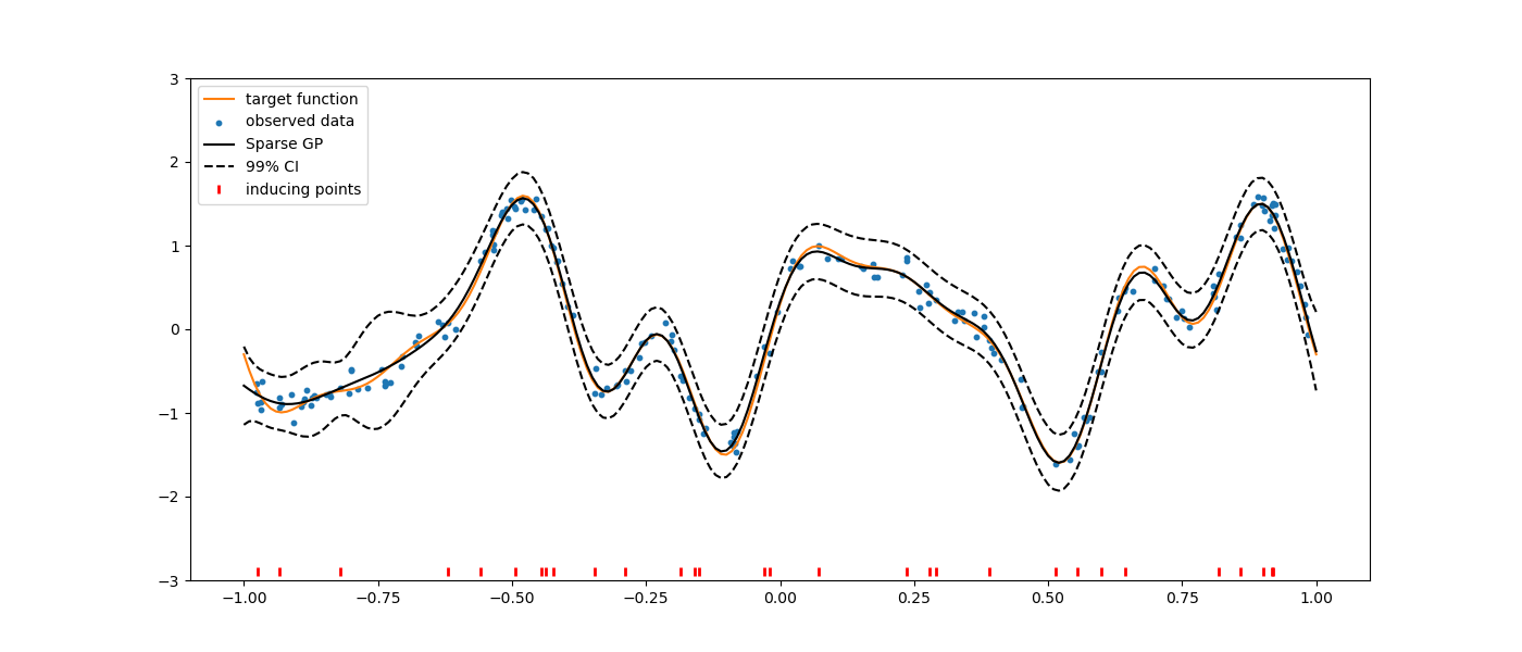
Using FITC method

import numpy as np
import matplotlib.pyplot as plt

from smt.surrogate_models import SGP

def f_obj(x):
    import numpy as np

    return (
        np.sin(3 * np.pi * x)
        + 0.3 * np.cos(9 * np.pi * x)
        + 0.5 * np.sin(7 * np.pi * x)
    )

# random generator for reproducibility
rng = np.random.RandomState(0)

# Generate training data
nt = 200
# Variance of the gaussian noise on our trainingg data
eta2 = [0.01]
gaussian_noise = rng.normal(loc=0.0, scale=np.sqrt(eta2), size=(nt, 1))
xt = 2 * rng.rand(nt, 1) - 1
yt = f_obj(xt) + gaussian_noise

# Pick inducing points randomly in training data
n_inducing = 30
random_idx = rng.permutation(nt)[:n_inducing]
Z = xt[random_idx].copy()

sgp = SGP()
sgp.set_training_values(xt, yt)
sgp.set_inducing_inputs(Z=Z)
# sgp.set_inducing_inputs()  # When Z not specified n_inducing points are picked randomly in traing data
sgp.train()

x = np.linspace(-1, 1, nt + 1).reshape(-1, 1)
y = f_obj(x)
hat_y = sgp.predict_values(x)
var = sgp.predict_variances(x)

# plot prediction
plt.figure(figsize=(14, 6))
plt.plot(x, y, "C1-", label="target function")
plt.scatter(xt, yt, marker="o", s=10, label="observed data")
plt.plot(x, hat_y, "k-", label="Sparse GP")
plt.plot(x, hat_y - 3 * np.sqrt(var), "k--")
plt.plot(x, hat_y + 3 * np.sqrt(var), "k--", label="99% CI")
plt.plot(Z, -2.9 * np.ones_like(Z), "r|", mew=2, label="inducing points")
plt.ylim([-3, 3])
plt.legend(loc=0)
plt.show()

___________________________________________________________________________

                                    SGP
___________________________________________________________________________

 Problem size

      # training points.        : 200

___________________________________________________________________________

 Training

   Training ...
   Training - done. Time (sec):  0.1044381
___________________________________________________________________________

 Evaluation

      # eval points. : 201

   Predicting ...
   Predicting - done. Time (sec):  0.0001109

   Prediction time/pt. (sec) :  0.0000006

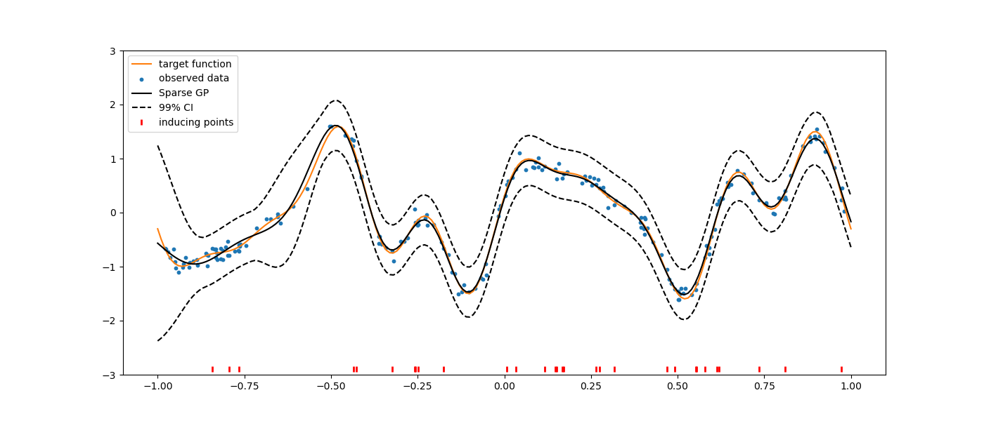
Using VFE method

import numpy as np
import matplotlib.pyplot as plt

from smt.surrogate_models import SGP

def f_obj(x):
    import numpy as np

    return (
        np.sin(3 * np.pi * x)
        + 0.3 * np.cos(9 * np.pi * x)
        + 0.5 * np.sin(7 * np.pi * x)
    )

# random generator for reproducibility
rng = np.random.RandomState(42)

# Generate training data
nt = 200
# Variance of the gaussian noise on our training data
eta2 = [0.01]
gaussian_noise = rng.normal(loc=0.0, scale=np.sqrt(eta2), size=(nt, 1))
xt = 2 * rng.rand(nt, 1) - 1
yt = f_obj(xt) + gaussian_noise

# Pick inducing points randomly in training data
n_inducing = 30
random_idx = rng.permutation(nt)[:n_inducing]
Z = xt[random_idx].copy()

sgp = SGP(method="VFE")
sgp.set_training_values(xt, yt)
sgp.set_inducing_inputs(Z=Z)
sgp.train()

x = np.linspace(-1, 1, nt + 1).reshape(-1, 1)
y = f_obj(x)
hat_y = sgp.predict_values(x)
var = sgp.predict_variances(x)

# plot prediction
plt.figure(figsize=(14, 6))
plt.plot(x, y, "C1-", label="target function")
plt.scatter(xt, yt, marker="o", s=10, label="observed data")
plt.plot(x, hat_y, "k-", label="Sparse GP")
plt.plot(x, hat_y - 3 * np.sqrt(var), "k--")
plt.plot(x, hat_y + 3 * np.sqrt(var), "k--", label="99% CI")
plt.plot(Z, -2.9 * np.ones_like(Z), "r|", mew=2, label="inducing points")
plt.ylim([-3, 3])
plt.legend(loc=0)
plt.show()

___________________________________________________________________________

                                    SGP
___________________________________________________________________________

 Problem size

      # training points.        : 200

___________________________________________________________________________

 Training

   Training ...
   Training - done. Time (sec):  0.0890281
___________________________________________________________________________

 Evaluation

      # eval points. : 201

   Predicting ...
   Predicting - done. Time (sec):  0.0001070

   Prediction time/pt. (sec) :  0.0000005

Options

List of options

Option	Default	Acceptable values	Acceptable types	Description
print_global	True	None	[‘bool’]	Global print toggle. If False, all printing is suppressed
print_training	True	None	[‘bool’]	Whether to print training information
print_prediction	True	None	[‘bool’]	Whether to print prediction information
print_problem	True	None	[‘bool’]	Whether to print problem information
print_solver	True	None	[‘bool’]	Whether to print solver information
poly	constant	[‘constant’]	[‘str’]	Regression function type
corr	squar_exp	[‘squar_exp’]	[‘str’]	Correlation function type
pow_exp_power	1.9	None	[‘float’]	Power for the pow_exp kernel function (valid values in (0.0, 2.0]), This option is set automatically when corr option is squar, abs, or matern.
categorical_kernel	MixIntKernelType.CONT_RELAX	[<MixIntKernelType.CONT_RELAX: ‘CONT_RELAX’>, <MixIntKernelType.GOWER: ‘GOWER’>, <MixIntKernelType.EXP_HOMO_HSPHERE: ‘EXP_HOMO_HSPHERE’>, <MixIntKernelType.HOMO_HSPHERE: ‘HOMO_HSPHERE’>, <MixIntKernelType.COMPOUND_SYMMETRY: ‘COMPOUND_SYMMETRY’>]	None	The kernel to use for categorical inputs. Only for non continuous Kriging
hierarchical_kernel	MixHrcKernelType.ALG_KERNEL	[<MixHrcKernelType.ALG_KERNEL: ‘ALG_KERNEL’>, <MixHrcKernelType.ARC_KERNEL: ‘ARC_KERNEL’>]	None	The kernel to use for mixed hierarchical inputs. Only for non continuous Kriging
nugget	2.220446049250313e-13	None	[‘float’]	a jitter for numerical stability
theta0	[0.01]	None	[‘list’, ‘ndarray’]	Initial hyperparameters
theta_bounds	[1e-06, 100.0]	None	[‘list’, ‘ndarray’]	bounds for hyperparameters
hyper_opt	Cobyla	[‘Cobyla’]	[‘str’]	Optimiser for hyperparameters optimisation
eval_noise	True	[True, False]	[‘bool’]	Noise is always evaluated
noise0	[0.01]	None	[‘list’, ‘ndarray’]	Gaussian noise on observed training data
noise_bounds	[2.220446049250313e-14, 10000000000.0]	None	[‘list’, ‘ndarray’]	bounds for noise hyperparameters
use_het_noise	False	[True, False]	[‘bool’]	heteroscedastic noise evaluation flag
n_start	10	None	[‘int’]	number of optimizer runs (multistart method)
xlimits	None	None	[‘list’, ‘ndarray’]	definition of a design space of float (continuous) variables: array-like of size nx x 2 (lower, upper bounds)
design_space	None	None	[‘BaseDesignSpace’, ‘list’, ‘ndarray’]	definition of the (hierarchical) design space: use smt.utils.design_space.DesignSpace as the main API. Also accepts list of float variable bounds
random_state	41	None	[‘NoneType’, ‘int’, ‘RandomState’]	Numpy RandomState object or seed number which controls random draws for internal optim (set by default to get reproductibility)
method	FITC	[‘FITC’, ‘VFE’]	[‘str’]	Method used by sparse GP model
n_inducing	10	None	[‘int’]	Number of inducing inputs