Sparse Multi-Fidelity Co-Kriging (SMFCK)

SMFCK is a multi-fidelity modeling method adding sparsity to the MFCK model. This model allows to add sparsity to all the fidelity levels.

We follow the same autoregressive formulation:

\[y_\text{high}({\bf x})=\rho(x) \cdot y_\text{low}({\bf x}) + \delta({\bf x})\]

where \(\rho(x)\) is a scaling/correlation factor (constant for MFCK) and \(\delta(\cdot)\) is a discrepancy function.

The additive AR1 formulation was first introduced by Kennedy and O’Hagan [1]. While MFK follows the recursive formulation of Le Gratiet [2]. SMFCK uses ab block-wise matrix construction for \(n\) levels of fidelity offering freedom in terms of data input assumptions. The sparse approximations are based on the formulations of Titsias [3] and given in [4].

References

[1]

Kennedy, M.C. and O’Hagan, A., Bayesian calibration of computer models. Journal of the Royal Statistical Society. 2001

[2]

Le Gratiet, L., Multi-fidelity Gaussian process regression for computer experiments. PhD Thesis. 2013

[3]

Titsias, M.K., Variational Learning of Inducing Variables in Sparse Gaussian Processes. In Proceedings of the 12th International Conference on Artificial Intelligence and Statistics (AISTATS), 2009

[4]

Castano-Aguirre, M., López-Lopera, F. A., Bartoli, N., Massa, F., & Lefebvre, T. Scalable Sparse Co-Kriging for Multi-Fidelity Data Fusion: An Application to Aerodynamics. Reliability Engineering & System Safety, 112485, 2026

Usage

import matplotlib.pyplot as plt
import numpy as np
from smt.sampling_methods import LHS  # noqa
from smt.applications import SMFCK

# low fidelity model
def lf_function(x):
    import numpy as np

    return (
        0.5 * ((x * 6 - 2) ** 2) * np.sin((x * 6 - 2) * 2)
        + (x - 0.5) * 10.0
        - 5
    )

# high fidelity model
def hf_function(x):
    import numpy as np

    return ((x * 6 - 2) ** 2) * np.sin((x * 6 - 2) * 2)

# Problem set up
xlimits = np.array([[0.0, 1.0]])
# Example with non-nested input data
Obs_HF = 7  # Number of observations of HF
Obs_LF = 14  # Number of observations of LF

# Creation of LHS for non-nested LF data
sampling = LHS(
    xlimits=xlimits,
    criterion="ese",
    seed=0,
)

xt_e_non = sampling(Obs_HF)
xt_c_non = sampling(Obs_LF)

# Evaluate the HF and LF functions
yt_e = hf_function(xt_e_non)
yt_c = lf_function(xt_c_non)

sm = SMFCK(
    hyper_opt="Cobyla",
    theta0=xt_e_non.shape[1] * [1.0],
    theta_bounds=[1e-6, 2.0],
    print_global=False,
    method="FITC",
    eval_noise=True,
    noise0=[1e-5],
    noise_bounds=np.array((1e-12, 10.0)),
    corr="squar_exp",
    n_inducing=[xt_c_non.shape[0] - 2, xt_e_non.shape[0] - 1],
)

# low-fidelity dataset names being integers from 0 to level-1
sm.set_training_values(xt_c_non, yt_c, name=0)
# high-fidelity dataset without name
sm.set_training_values(xt_e_non, yt_e)

# train the model
sm.train()

x = np.linspace(0, 1, 101, endpoint=True).reshape(-1, 1)

# query the outputs

mean, cov = sm.predict_all_levels(x)

y = mean[-1]
# _derivs = sm.predict_derivatives(x, kx=0)

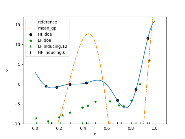
plt.figure()

plt.plot(x, hf_function(x), label="reference")
plt.plot(x, y, linestyle="-.", label="mean_gp")
plt.scatter(xt_e_non, yt_e, marker="o", color="k", label="HF doe")
plt.scatter(xt_c_non, yt_c, marker="*", color="g", label="LF doe")
plt.plot(
    sm.Z[0],
    -9.9 * np.ones_like(sm.Z[0]),
    "g|",
    mew=2,
    label=f"LF inducing:{sm.Z[0].shape[0]}",
)
plt.plot(
    sm.Z[1],
    -9.9 * np.ones_like(sm.Z[1]),
    "k|",
    mew=2,
    label=f"HF inducing:{sm.Z[1].shape[0]}",
)

plt.legend(loc=0)
plt.ylim(-10, 17)
plt.xlim(-0.1, 1.1)
plt.xlabel(r"$x$")
plt.ylabel(r"$y$")

plt.show()

Options

List of options

Option	Default	Acceptable values	Acceptable types	Description
print_global	True	None	[‘bool’]	Global print toggle. If False, all printing is suppressed
print_training	True	None	[‘bool’]	Whether to print training information
print_prediction	True	None	[‘bool’]	Whether to print prediction information
print_problem	True	None	[‘bool’]	Whether to print problem information
print_solver	True	None	[‘bool’]	Whether to print solver information
poly	constant	[‘constant’, ‘linear’, ‘quadratic’]	[‘str’]	Regression function type
corr	squar_exp	[‘pow_exp’, ‘abs_exp’, ‘squar_exp’, ‘matern52’, ‘matern32’]	[‘str’, ‘Kernel’]	Correlation function type
pow_exp_power	1.9	None	[‘float’]	Power for the pow_exp kernel function (valid values in (0.0, 2.0]). This option is set automatically when corr option is squar, abs, or matern.
categorical_kernel	MixIntKernelType.CONT_RELAX	[<MixIntKernelType.CONT_RELAX: ‘CONT_RELAX’>, <MixIntKernelType.GOWER: ‘GOWER’>, <MixIntKernelType.EXP_HOMO_HSPHERE: ‘EXP_HOMO_HSPHERE’>, <MixIntKernelType.HOMO_HSPHERE: ‘HOMO_HSPHERE’>, <MixIntKernelType.COMPOUND_SYMMETRY: ‘COMPOUND_SYMMETRY’>, <MixIntKernelType.DIST_ENCODING: ‘DIST_ENCODING’>]	None	The kernel to use for categorical inputs. Only for non continuous Kriging
categorical_kernel_beta	1.0	None	[‘float’, ‘int’]	Power for the distributional encoding kernel (valid values in (0.0, 2.0]).
hierarchical_kernel	MixHrcKernelType.ALG_KERNEL	[<MixHrcKernelType.ALG_KERNEL: ‘ALG_KERNEL’>, <MixHrcKernelType.ARC_KERNEL: ‘ARC_KERNEL’>]	None	The kernel to use for mixed hierarchical inputs. Only for non continuous Kriging
nugget	2.220446049250313e-13	None	[‘float’]	a jitter for numerical stability
theta0	[0.01]	None	[‘list’, ‘ndarray’]	Initial hyperparameters
theta_bounds	[1e-06, 20.0]	None	[‘list’, ‘ndarray’]	bounds for hyperparameters
hyper_opt	Cobyla	[‘Cobyla’, ‘Cobyla-nlopt’]	None	Optimiser for hyperparameters optimisation
eval_noise	False	[True, False]	[‘bool’]	If True, the model evaluates noise variance, can be homoscedastic or heteroscedastic
noise0	[0.0]	None	[‘list’, ‘ndarray’]	Initial noise hyperparameters
noise_bounds	[np.float64(2.220446049250313e-14), 10000000000.0]	None	[‘list’, ‘ndarray’]	bounds for noise hyperparameters
use_het_noise	False	[True, False]	[‘bool’]	If True, the model considers Heteroscedastic noise, array with the same size of y(x) is expected
n_start	10	None	[‘int’]	number of optimizer runs (multistart method)
xlimits	None	None	[‘list’, ‘ndarray’]	definition of a design space of float (continuous) variables: array-like of size nx x 2 (lower, upper bounds)
design_space	None	None	[‘BaseDesignSpace’, ‘list’, ‘ndarray’]	definition of the (hierarchical) design space: use smt.design_space.DesignSpace as the main API. Also accepts list of float variable bounds
is_ri	False	None	[‘bool’]	activate reinterpolation for noisy cases
seed	0	None	[‘NoneType’, ‘int’]	seed number which controls random draws
predict_with_noise	False	[True, False]	[‘bool’]	if use_het_noise is true, then the prediction of the noise variance over the test set will given
rho0	1.0	None	[‘float’]	Initial rho for the autoregressive model , (scalar factor between two consecutive fidelities, e.g., Y_HF = (Rho) * Y_LF + Gamma
rho_bounds	[-5.0, 5.0]	None	[‘list’, ‘ndarray’]	Bounds for the rho parameter used in the autoregressive model
sigma0	1.0	None	[‘float’]	Initial variance parameter
sigma_bounds	[1e-06, 100]	None	[‘list’, ‘ndarray’]	Bounds for the variance parameter
lambda	0.0	None	[‘float’]	Regularization parameter
n_inducing	[6, 5]	None	[‘list’, ‘ndarray’]	Number of inducing points per fidelity level
method	FITC	[‘FITC’]	[‘str’]	Methods available for Sparse Multi-fidelity
inducing_method	kmeans	[‘random’, ‘kmeans’]	[‘str’]	The chosen method to induce points