Knowledge-enhanced radial basis functions
The effectiveness of surrogate models is often limited by data scarcity. One way to improve the performance of such surrogate models is by leveraging domain-specific knowledge to guide model predictions. RBF-Gen [1] is a radial basis function (RBF)-based generative model that allows for the integration of domain-specific knowledge in surrogate models without affecting data interpolation. First an RBF model is constructed
where \(\mathbf{x} \in \mathbb{R}^{n_x}\) is the prediction input vector, \(y \in \mathbb{R}\) is the prediction output, \(\phi(\mathbf{x}, \mathbf{xf}_i) \in \mathbb{R}\) is a radial basis function kernel, \(\mathbf{xf}_i \in \mathbb{R}^{nx}\) is the location of the center of the \(i\) th radial kernel, and \(w_i \in \mathbb{R}\) are the radial basis function coefficients. Enforcing interpolation of \(nt\) data points \(\mathbf{yt}_i \in \mathbb{R}\) at corresponding input vectors \(\mathbf{xt}_i \in \mathbb{R}^{nx}\) with \(K\) radial kernels results in the following linear system,
where \(\Phi \in \mathbb{R}^{nt \times K}\). For \(K > nt\) this system is underdetermined and does not have a unique solution. We use a least-squares approach to compute the minimum-norm solution \(\mathbf{w}_0\),
and compute an orthonormal basis \(N \in \mathbb{R}^{K \times K - nt}\) for the nullspace of \(\Phi\).
The radial basis function weight vector \(\mathbf{w} = \mathbf{w}_0 + N \mathbf{\alpha}\), with \(\mathbf{\alpha} \in \mathbb{R}^{K-nt}\), interpolates the given data points for any \(\mathbf{\alpha}\). We train a neural network generator \(G\) to map latent variables \(z \sim \mathcal{N}(0, 1)^d\), with \(d\) the dimension of the latent space, into coefficient vectors \(\mathbf{\alpha}\), such that the interpolant with the resultant weight vector \(\mathbf{w} = \mathbf{w}_0 + N \mathbf{\alpha}\) is consistent with domain-specific knowledge. To this end, the generator \(G\) is trained to minimize one or more loss terms. Every training epoch we sample a batch of latent variables \(z \sim \mathcal{N}(0, 1)^d\). Several types of loss terms are implemented in SMT:
Monotonicity: We know that the underlying model increases (decreases) monotonically under input changes, and therefore penalize negative (positive) derivatives.
Positivity: We know that the output quantity is always positive, and therefore penalize negative output values.
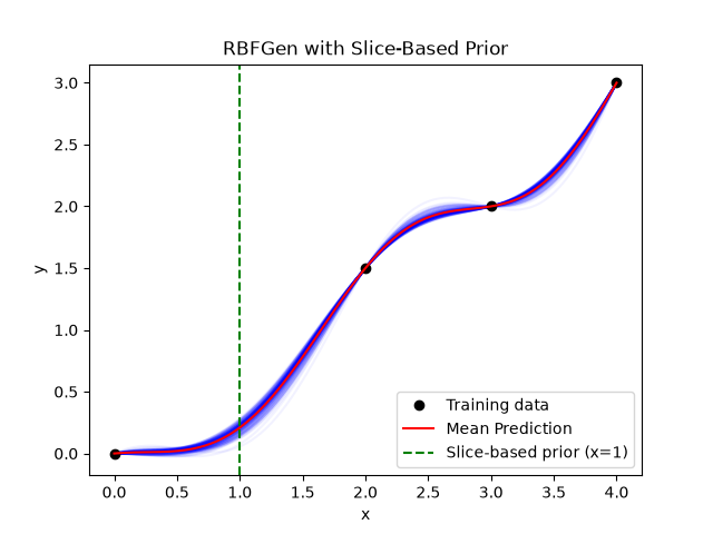
Slice-based priors: We know the output mean and standard deviation in one or more points, for example from experimental data. We therefore penalize deviations from this imposed output mean and standard deviation of the batch of outputs \(\mathbf{w} = \mathbf{w}_0 + N \mathbf{\alpha}(z)\).
A base LossTerm class is available, which can be used to create custom loss terms. A non-exhaustive list of examples can be found in [1].
Usage
Example 1, with monotonicity and positivity loss terms
import matplotlib.pyplot as plt
import numpy as np

from smt.surrogate_models import RBFGen
from smt.utils.nn_lossterms import MonotonicityLossTerm, PositivityLossTerm
from smt.utils.nn_rich_rbf import rbf_features

xt = np.array([[0.0], [2.0], [3.0], [4.0]])
yt = np.array([[0.0], [1.5], [2.0], [3.0]])

sm = RBFGen(epochs=500, learning_rate=5e-2, rbf_m_centers=50)
sm.set_training_values(xt, yt)

sm.add_loss_term(MonotonicityLossTerm(x_train=xt, random_base_points=True))
sm.add_loss_term(PositivityLossTerm(x_train=xt))
sm.train()

num = 100
x = np.linspace(0.0, 4.0, num).reshape(-1, 1)
y = sm.predict_values(x)
s2 = sm.predict_variances(x)
s2 = s2[:, 0]

plt.figure()
rbf = sm.options["rbf_surrogate"]
Phi_q = rbf_features(x, rbf.rbf_centers, rbf.d0)
y_ensemble = sm.network_weights @ Phi_q.T
for i in range(y_ensemble.shape[0]):
    plt.plot(x, y_ensemble[i, :], alpha=0.05, color='blue')
plt.plot(xt, yt, "o", color='black', label="Training data")
plt.plot(x, y, color='red', label="Mean Prediction")
plt.xlabel("x")
plt.ylabel("y")
plt.title("RBFGen")
plt.legend()
plt.show()
___________________________________________________________________________

                                  RBFGen
___________________________________________________________________________

 Problem size

      # training points.        : 4

___________________________________________________________________________

 Training

   Training ...
___________________________________________________________________________

                                 NNRichRBF
___________________________________________________________________________

 Problem size

      # training points.        : 4

___________________________________________________________________________

 Training

   Training ...
   Training - done. Time (sec):  0.0009499
Epoch   100/500 | Total Loss: 9.6226e-05 | MonotonicityLossTerm: 1.0189e-09 | PositivityLossTerm: 9.6225e-05
Epoch   200/500 | Total Loss: 9.5401e-05 | MonotonicityLossTerm: 1.0459e-09 | PositivityLossTerm: 9.5400e-05
Epoch   300/500 | Total Loss: 9.4618e-05 | MonotonicityLossTerm: 1.2594e-09 | PositivityLossTerm: 9.4616e-05
Epoch   400/500 | Total Loss: 9.4926e-05 | MonotonicityLossTerm: 1.8646e-09 | PositivityLossTerm: 9.4924e-05
Epoch   500/500 | Total Loss: 9.4423e-05 | MonotonicityLossTerm: 2.4403e-09 | PositivityLossTerm: 9.4420e-05
   Training - done. Time (sec):  1.0252733
___________________________________________________________________________

 Evaluation

      # eval points. : 100

   Predicting ...
   Predicting - done. Time (sec):  0.0001841

   Prediction time/pt. (sec) :  0.0000018

___________________________________________________________________________

 Evaluation

      # eval points. : 100

   Predicting ...
   Predicting - done. Time (sec):  0.0001655

   Prediction time/pt. (sec) :  0.0000017

Example 2, with monotonicity, positivity and slice-based prior loss terms
import matplotlib.pyplot as plt
import numpy as np

from smt.surrogate_models import RBFGen
from smt.utils.nn_lossterms import MonotonicityLossTerm, PositivityLossTerm, SliceBasedPriorLossTerm
from smt.utils.nn_rich_rbf import rbf_features

xt = np.array([[0.0], [2.0], [3.0], [4.0]])
yt = np.array([[0.0], [1.5], [2.0], [3.0]])

prior_points = np.array([[1.0]])
prior_means = np.array([0.2])
prior_stds = np.array([0.05])

sm = RBFGen(epochs=1000, learning_rate=5e-2, rbf_m_centers=50)
sm.set_training_values(xt, yt)

sm.add_loss_term(MonotonicityLossTerm(x_train=xt, random_base_points=True))
sm.add_loss_term(PositivityLossTerm(x_train=xt))
sm.add_loss_term(SliceBasedPriorLossTerm(x_train=xt, prior_points=prior_points,
                                         prior_means=prior_means, prior_stds=prior_stds,
                                         loss_term_weight=1.))
sm.train()

num = 100
x = np.linspace(0.0, 4.0, num).reshape(-1, 1)
y = sm.predict_values(x)
s2 = sm.predict_variances(x)
s2 = s2[:, 0]

plt.figure()
rbf = sm.options["rbf_surrogate"]
Phi_q = rbf_features(x, rbf.rbf_centers, rbf.d0)
y_ensemble = sm.network_weights @ Phi_q.T
for i in range(y_ensemble.shape[0]):
    plt.plot(x, y_ensemble[i, :], alpha=0.05, color='blue')
plt.plot(xt, yt, "o", color='black', label="Training data")
plt.plot(x, y, color='red', label="Mean Prediction")
plt.axvline(1.0, color='green', linestyle='--', label="Slice-based prior (x=1)")
plt.xlabel("x")
plt.ylabel("y")
plt.title("RBFGen with Slice-Based Prior")
plt.legend()
plt.show()
___________________________________________________________________________

                                  RBFGen
___________________________________________________________________________

 Problem size

      # training points.        : 4

___________________________________________________________________________

 Training

   Training ...
___________________________________________________________________________

                                 NNRichRBF
___________________________________________________________________________

 Problem size

      # training points.        : 4

___________________________________________________________________________

 Training

   Training ...
   Training - done. Time (sec):  0.0005474
Epoch   100/1000 | Total Loss: 1.2562e-02 | MonotonicityLossTerm: 5.6323e-16 | PositivityLossTerm: 1.1543e-02 | SliceBasedPriorLossTerm: 1.0192e-03
Epoch   200/1000 | Total Loss: 1.1136e-02 | MonotonicityLossTerm: 1.2610e-13 | PositivityLossTerm: 8.9831e-03 | SliceBasedPriorLossTerm: 2.1533e-03
Epoch   300/1000 | Total Loss: 1.0373e-02 | MonotonicityLossTerm: 3.3316e-10 | PositivityLossTerm: 8.0135e-03 | SliceBasedPriorLossTerm: 2.3594e-03
Epoch   400/1000 | Total Loss: 9.4484e-03 | MonotonicityLossTerm: 1.3334e-15 | PositivityLossTerm: 6.7688e-03 | SliceBasedPriorLossTerm: 2.6796e-03
Epoch   500/1000 | Total Loss: 8.4162e-03 | MonotonicityLossTerm: 2.3027e-08 | PositivityLossTerm: 6.2890e-03 | SliceBasedPriorLossTerm: 2.1272e-03
Epoch   600/1000 | Total Loss: 7.3066e-03 | MonotonicityLossTerm: 8.5274e-10 | PositivityLossTerm: 5.0991e-03 | SliceBasedPriorLossTerm: 2.2075e-03
Epoch   700/1000 | Total Loss: 6.1193e-03 | MonotonicityLossTerm: 7.6946e-10 | PositivityLossTerm: 4.5380e-03 | SliceBasedPriorLossTerm: 1.5813e-03
Epoch   800/1000 | Total Loss: 5.1085e-03 | MonotonicityLossTerm: 1.9992e-12 | PositivityLossTerm: 3.3375e-03 | SliceBasedPriorLossTerm: 1.7710e-03
Epoch   900/1000 | Total Loss: 4.0144e-03 | MonotonicityLossTerm: 5.2812e-08 | PositivityLossTerm: 3.0393e-03 | SliceBasedPriorLossTerm: 9.7513e-04
Epoch  1000/1000 | Total Loss: 3.1242e-03 | MonotonicityLossTerm: 9.6583e-08 | PositivityLossTerm: 2.2126e-03 | SliceBasedPriorLossTerm: 9.1151e-04
   Training - done. Time (sec):  1.3454084
___________________________________________________________________________

 Evaluation

      # eval points. : 100

   Predicting ...
   Predicting - done. Time (sec):  0.0001571

   Prediction time/pt. (sec) :  0.0000016

___________________________________________________________________________

 Evaluation

      # eval points. : 100

   Predicting ...
   Predicting - done. Time (sec):  0.0001385

   Prediction time/pt. (sec) :  0.0000014
Options
Option |
Default |
Acceptable values |
Acceptable types |
Description |
|---|---|---|---|---|
print_global |
True |
None |
[‘bool’] |
Global print toggle. If False, all printing is suppressed |
print_training |
True |
None |
[‘bool’] |
Whether to print training information |
print_prediction |
True |
None |
[‘bool’] |
Whether to print prediction information |
print_problem |
True |
None |
[‘bool’] |
Whether to print problem information |
print_solver |
True |
None |
[‘bool’] |
Whether to print solver information |
rbf_surrogate |
None |
None |
[‘NNRichRBF’, ‘NoneType’] |
The RBF surrogate object |
rbf_m_centers |
None |
None |
[‘int’, ‘NoneType’] |
Number of RBF centers. If None, defaults to max(3*[number of training points], 100). |
rbf_d0 |
None |
None |
[‘float’, ‘int’, ‘NoneType’] |
RBF width (epsilon). If None, computed via median heuristic. |
rbf_rng_seed |
1 |
None |
[‘int’, ‘Generator’, ‘NoneType’] |
Random seed or generator for center selection. |
rbf_centers_distribution |
random |
[‘random’, ‘linspace’] |
None |
Distribution of RBF centers: ‘random’ (uniform random) or ‘linspace’ (regular grid). |
learning_rate |
0.001 |
None |
[‘float’] |
Learning rate for the network optimizer |
alpha_scale |
1.0 |
None |
[‘float’] |
Scaling factor for alpha |
epochs |
1000 |
None |
[‘int’] |
Number of training epochs |
batch_size |
64 |
None |
[‘int’] |
Batch size for training |
latent_space_dim |
12 |
None |
[‘int’] |
Dimension of the latent space |
num_eval_pts |
100 |
None |
[‘int’] |
Number of evaluation points for nullspace |